This is a guide to the TRIM.FaTE Computer Framework. This document is accessible in the doc subdirectory of the TRIM installation directory under the file name user_guide.html. Background and other information about TRIM.FaTE and the TRIM project as a whole can be found in the following documents:
Exceptions: Exceptions are errors that are detected when a program is executing. In TRIM.FaTE, exceptions are used to notify you of problems. Exceptions are often presented to you with a dialog box that shows the name of the exception and the message that was passed with it. The name is sometimes preceded by a Java package, such as java.io.IOException, or gov.epa.trim.util.TRIMException.
Object: A general term that refers to items created and used by TRIM.FaTE. Examples include: Volume Elements, Chemicals, Compartments, Links, Algorithms, Sources, Property Types, Sinks, and Scenarios.
Library: A repository for different types of objects that can be drawn upon for use in modeling scenarios. Libraries and their contents can be saved to disk. The following types of objects are stored in libraries: Algorithms, Chemicals, Compartments, Composite Compartments, Sources, and Property Types.
Project: Contains a collection of modeling scenarios and references a set of libraries whose objects can be used by the scenarios. Projects and their contents can be saved to disk.
Scenario: A configuration for a simulation that includes properties such as the starting date/time, ending date/time, and all the information that constitutes the outdoor environment.
Outdoor Environment: The environment that is used for a simulation. This includes the volume elements used, their compartments, links, and algorithms; and the chemicals, sources, and sinks used.
Property: Objects have properties that store information about the objects in the system. Examples of properties for a chemical include melting point, vapor pressure, and molecular weight; examples of properties for an algorithm include the receiving compartment type, sending compartment type, and whether it transforms a chemical. Each property references a property type that defines the name of the property, the type of data (e.g., real number, date and time, true or false), a default value, a description, and for numeric data types the recommended minimum and maximum values and the units. Objects have some properties that are always present (mandatory) and others that are optional. For more information on mandatory and optional properties for each type of object, see the Object Importer Specification.
Property Type: Each property has a single property type that defines the name, type of data, units, default value, and minimum and maximum values for the property. The available types of data are: real number, integer, date and time, true or false, text, and category.
Category: A hierarchical classification for objects ordered from most general to most specific, with each level separated by a vertical bar ("|"). For example, a chemical might have a category of "metal" or "organic | aldehyde"; a biological organism might have a category of "bird" or "mammal | rodent". There is an implicit category called "All" that all other categories are more specific than. This is useful in cases where a category is used to specify which objects are applicable for a certain purpose. For example, if "All" is the value of the acceptableAbiotic property for a compartment, then the compartment can be attached to a volume element with any type of abiotic compartment, or if "All" is the value of the chemicalCategory property for an algorithm, it means the algorithm is applicable to all chemicals.
Form: A property that stores data of type Real Number can come in several different "forms", such as "Constant Real Number" (a singular value), "Unevenly Time Stepped Real Number" (a sequence of real values with associated dates and times), or Formula Real Number (a mathematical formula that can include references to other properties in this or other objects).
Composite Compartment: A composite compartment is a compartment
that is made up of other compartments. For example,
leaves, a stem, and roots may comprise a plant.
To use TRIM.FaTE, your PC should be equipped with at least:
PCs with lesser configurations will also work, but performance (e.g., model run time) will be less than optimal.
Software Requirements
TRIM.FaTE is compatible with the following computer operating systems:
However, Windows XP, Windows 2000, and Windows NT are the recommended operating systems for running TRIM.FaTE because they best meet the memory requirements of the model. Because TRIM.FaTE was developed using Java, it can be run under a number of other operating systems, such as Linux and Solaris; however, TRIM.FaTE has not been fully implemented or tested in any non-Windows-based operating systems to date.
Important Note: If installing TRIM.FaTE on a computer using the Windows XP, Windows 2000, or Windows NT operating system, the user must be logged onto the computer as an "Administrator" to complete the installation process. If it is not clear how to do this, contact the person(s) in charge of maintaining software on your computer.
FaTE is now installed as part of the larger TRIM system. For the latest installation instructions, please see those available from the TRIM Installation page under the web site http://www.epa.gov/ttn/fera. The instructions may also be available from your local TRIM installation at ../install.html.
Once the TRIM.FaTE installation is complete, the system is ready to run. TRIM.FaTE is started by running the trimjava.bat file, as described below.
After starting TRIM, the user should set the user and system paths, as described below.
Figure 2. Selecting Preferences
Note that the on-line Computer Framework Guide may not be available from the Help menu until TRIM.FaTE has been restarted after setting the preferences.
Several problems that have arisen in TRIM.FaTE test applications are listed in Table 1 along with solutions or suggested methods for circumventing the problem. Note that this list is not meant to be comprehensive and focuses primarily on general problems related to navigation of the TRIM.FaTE software that users have encountered in test case applications.
Table 1. Common TRIM.FaTE Problems and Suggested Solutions
|
Problem |
Description |
Solution |
|
TRIM.FaTE runs very slowly in Windows 98. |
In Windows 98, Java experiences problems releasing memory that is no longer needed, causing the program to slow down. |
Exit from TRIM.FaTE and/or reboot. Use the System Monitor tool in Windows 98 to keep track of the amount of memory used. The System Monitor is found in the Start menu-Programs-Accessories-System Tools. |
|
The trimjava.bat file will not run. |
When running trimjava.bat, the message "Out of environment space" appears. |
There are two ways to fix this problem: (1) Open the MS-DOS Command Prompt window under Programs in the Start Menu. From the bar at the top of the window that appears, click the right mouse button to bring up a menu and choose Properties. In the Memory tab, set the Initial Environment item to "1024." (2) For Windows 95/98, add the following line to the config.sys file using a text editor: shell=C:\COMMAND.COM /p /e:1024 For Windows NT, include the following line in the config.nt file using a text editor: shell=%systemroot%\system32\COMMAND. COM /p /e:1024 In both examples, 1024 is the maximum length in bytes that COMMAND.COM will allocate for each program. The default is 256 bytes, and the maximum is 32,000 K. Note: Other options may be set for the shell on your computer that are not shown here. These items will also be included in the revised shell line in your system configuration and do not need to be altered. |
|
The on-line computer framework guide does not take me to the section for which I want help. |
The first time the computer framework guide is accessed from the Help menu after TRIM.FaTE has been started, the user is sent to the beginning of the users guide instead of the section specific to the window currently in use. |
Use the Table of Contents to access the section of interest, or close the users guide and reload it. The guide will now send you to the proper section from the Help menu. |
|
A window does not move to the front when I click on it. |
Clicking on a window in the "background" does not bring the window to the "front." |
This is a problem with one of the Java or Windows toolkits used by TRIM.FaTE. Click on another window, and then click on the original window to prompt it to move to the front. |
|
Window splitters do not work properly. |
Window splitters calculate the minimum size of the items on either side and will not reduce items beyond their minimum size. |
Enlarge the window containing the window to be split before using the splitter, or use the buttons at the top of the splitter to move it completely to one side of the window. |
|
The Value column in the Library Property Editor appears to be missing. |
When showing properties for a chemical in a library, the Chemical column is removed because properties for chemicals cannot be chemical-dependent. The Value column may appear to be missing when you switch to another type of object after showing Chemical properties. |
The Value column is actually on the right side of the table. Scroll to the right and move the column to the desired position by grabbing its Title Bar and dragging it to the appropriate place. |
|
Object windows do not close with the project/library. |
The object windows that are open do not close when the project is closed. |
If Object windows are open when a project/library is closed, the Object window will remain open. Use the Close All button from the File drop down menu to close all windows. |
|
Library file size increases unexpectedly. |
In some cases, users have noticed instances when the library file size suddenly becomes significantly larger, even though a lot of objects have not been added. |
Currently, the cause of this problem is unknown. TRIM.FaTE users are encouraged to contact EPA if they are able to determine a specific situation where this problem can be reproduced. |
|
TRIM.FaTE will not close by clicking the "X" in the upper right-hand corner of the screen |
Closing TRIM.FaTE by clicking the "X" in the upper right-hand corner is unsuccessful. If one of the TRIM.FaTE windows is maximized within the main TRIM.FaTE window, TRIM.FaTE will only close the interior window when the "X" for the main TRIM.FaTE window is clicked. |
To close TRIM.FaTE completely, the user must press the "X" in the main TRIM.FaTE window twice, or select "Close All" from the "File" menu for the main TRIM.FaTE window. |
| Menu Item | Operation |
| File - New Project | Create a new project |
| File - Open Project | Open an existing project |
| File - Most Recently Opened Project | Open the most recently opened project |
| File - New Library | Create a new library |
| File - Open Library | Open an existing library |
| File - Most Recently Opened Library | Open the most recently opened library |
| File - Close All | Close all windows open in TRIM.FaTE |
| File - Preferences | Set preferences for running TRIM.FaTE (e.g., installation directory, MySQL username and password, and TRIM.FaTE user directory). |
| File - Exit FaTE | Close TRIM.FaTE and all its windows |
| Edit - Undo | Undo the last operation (where available) |
| Edit - Redo | Redo the last operation (where available) |
| Windows | Shows a list of all open windows; go to a particular window by choosing from the list |
| Help - TRIM.FaTE Computer Framework Guide | Show this computer framework guide |
| Help - About | Gives basic information about the TRIM.FaTE version |
From this window you can create new or examine existing objects. The window has three parts: the menu bar at the top, the object browser on the left, and the Property Editor on the right. The Property Editor is discussed in a later section. The functions of the object browser and menu bar are described in Table 3. The objects that currently exist in the library of the class specified by Contents are shown in a list below the Contents menu. The list will have scroll bars if needed. You can select objects from this list (and from many other lists & tables in the system) in several ways:
If you need to change the relative sizes of the left and right sides of the Library Window, place the mouse pointer on the boundary between the left and right parts of the window so that a double arrow appears, then Click and drag the divider to the left or right. This type of graphical user interface (GUI) feature is called a "splitter". You can make one side or the other of the window totally disappear by putting the mouse pointer over one of the small arrows near the top of the splitter, and doing a single click with the left mouse button. Splitters are used in several parts of the TRIM.FaTE GUI.
| Item or Button Name | Operation |
| Contents | Select the class of object to work with. To choose a new class, click on the down arrow. The available choices are Algorithms, Chemicals, Compartments, Composite Compartments, Sources, and Property Types. |
| Select | Select all objects that contain a string; you are prompted for the string to search for |
| Properties | Show the properties for all the selected objects in the Property Editor to the right. |
| Open | Open editors (usually object windows) for each of the selected objects |
| Delete | Delete all the selected objects |
| New | Create a new object of the type currently selected in the Contents menu |
| Duplicate | Make duplicate copies of all the selected objects; you are prompted to name each of the duplicates |
| File - Open Library | Open another library; you are prompted with a file browser |
| File - Import | Import objects to the library from a file; you are prompted for the type of importer to use (the Object Importer and Property Type Spreadsheet Importer are currently available), and then to choose a file to import using a file browser |
| File - Export | Export all objects in the library to a file; you are prompted for the type of exporter to use (the Object Exporter, Property Exporter, and Property Type Exporter are currently available), and then to choose a file to write to using a file browser |
| File - Export Selected | Export only the currently selected objects in the library to a file; you are prompted for the type of exporter to use (the Object Exporter, Property Exporter, and Property Type Exporter are currently available), and then to choose a file to write to using a file browser |
| File - Save Library | Save this library to a file using its current file name (or you are prompted to choose a file name if this is a newly created library) |
| File - Save Library As | Save this library to a new file name |
| File - Close Library | Close this library |
| File - Close All | Close all open windows |
| Edit - Undo | Undo the last operation (when available) |
| Edit - Redo | Redo the last operation (when available) |
| Edit - Edit Library Description | Edit the textual description of the library |
| Help | Get help on TRIM.FaTE |
The Property Editor has three parts: the label and button bar at the top, the property table in the center, and the Value Editor at the bottom. The Value Editor is used only for the special formula and time-stepped properties mentioned above; values for other types of properties are edited directly in the table. Note that there is a splitter between the property table and the Value Editor. The buttons for the Property Editor and Value Editor are described in Table 4.
The property table shows all the properties in the object(s) for which the Property Editor was created. For example, from the Library Window you can select multiple objects and then click the "Properties" button. This shows you the properties for all objects selected in the library's list in the Property Editor. Using the property table to edit multiple objects is very powerful because it allows you to add, delete, or modify properties for many objects simultaneously. The values for the properties are compared and if they are all the same, the actual value is shown in the Value column. If they are not all the same, "<Differ>" is shown as the value. If the property does not exist for all selected objects, "<Not in all>" is shown as the value. If a property is not in all selected objects and you want to put it in all selected objects, first delete the property, then add it back using the "New" button. The label at the top of the Property Editor indicates whether one or multiple objects are being edited by modifying the case of the object class and listing the names of multiple objects as space allows (e.g., "Properties for Algorithm a" vs. "Properties for 3 Algorithms a, b, c"). Some additional information about the property table follows:
| Button | Operation |
| New | Create new properties. You are prompted to select one or more property types to create properties for, and a single chemical that the new properties apply to. The system then creates new properties for each selected property type using the selected chemical; if the editor is editing multiple objects, the new properties are added to each object |
| Del | Delete all selected properties from the objects this editor is for |
| Desc | Open windows that contain the descriptions for all selected properties |
| PType | Open the Property Type Windows for all selected properties |
| Form | For real number properties, you are prompted to select the new form of the property. The available forms are a constant, a formula, or a series of time-stepped values. This option has no effect for properties that are not real numbers. |
| Undo | Undo the last operation (when available) |
| Redo | Redo the last operation (when available) |
| Insert | Insert a new time/value pair for an unevenly time-stepped property; the new row is placed after the currently selected row |
| Delete | Delete all selected rows for an unevenly time-stepped property |
| Store | Store the contents of the formula or unevenly time-stepped property with the property; until Store is pressed, any changes made will not be kept with the property |
| Import | You are prompted for a text file from which values will be imported
into an unevenly time-stepped property. Files to be imported should have
the following format: date (dd/mm/yyyy), hour, time zone (e.g. EST), value
(fields are separated by tabs or other white space and comment lines
are preceded with the # character). Data does not need to be given
at regular intervals and is treated as a step function in intervening
periods. For example:
# Level 1 Wind speed data from the National Weather Service # DD/MM/YYYY Hour TimeZone Value (m/s) 01/1/1991 0 EST 6.826 01/2/1991 0 EST 5.993 |
| Sort | Sort the entries for an unevenly time-stepped property by date and time. |
| Help | Show a help window for the Value Editor |
| Menu Item | Operation |
| File - Close Window | Close this window |
| File - Close All | Closes all windows open in TRIM.FaTE |
| Edit - Undo | Undo the last operation (where available) |
| Edit - Redo | Redo the last operation (where available) |
| Edit - Rename | Rename this object |
| Edit - Description | Edit the description of this object |
| Help | Get help on TRIM.FaTE |
New property types with the following names should not be created, as
they are standard names with special meanings to the system:
mass, moles, totalMass, initialConcentration_g_per_m3, initialConcentration_g_per_L,
initialConcentration_g_per_kg, boundaryConcentration_g_per_m3, emissionRate,
useSpecifiedConcentration, concentration_g_per_m3, concentration_g_per_L,
concentration_g_per_kg, boundaryContribution.
| Item or Button Name | Function |
| FaTE... (Scenarios) | Opens Fate Scenario windows for the selected scenarios these windows are discussed in the next subsection) |
| Expo... (Scenarios) | Opens Expo Scenario windows for the selected scenarios (these windows are discussed below) |
| New (Scenarios) | Create a new scenario in the project; you are prompted to name the scenario |
| Delete | Delete the selected scenarios |
| Rename | Rename the selected scenario; you are prompted for a new name |
| Duplicate | Duplicate the selected scenarios; you are prompted for the new name(s); the new scenario is noted to be derived from the original scenario |
| Open (Libraries) | Opens the selected libraries in Library Windows |
| Remove | Removes the selected libraries from the project |
| New (Libraries) | Creates a new library; you are prompted about whether to add it to the project |
| Add | Add a library to the project; a file browser is provided to select a library |
| File - Open Project | Open another project; you are prompted with a file browser |
| File - Save Project | Save this project to a file using its current file name (or you are prompted to choose a file name if this is a newly created project) |
| File - Save Project As | Save this project to a new file name |
| File - Close Project | Close this project |
| File - Close All | Close all open windows |
| Edit - Undo | Undo the last operation (when available) |
| Edit - Redo | Redo the last operation (when available) |
| Edit - Edit Project Description | Edit the textual description of the project |
| Help | Get help on TRIM.FaTE |
When you select a scenario in a project and click the "FaTE..." button beneath the Scenarios list, a FaTE Scenario Window appears for the selected scenario. This window provides you access to many functions that must be performed before running a TRIM.FaTE simulation. The window consists of a menu bar and a set of tabbed views that allow you to define the properties of the scenario and its outdoor environment. There is a tab for the scenario and one tab each for the sources, chemicals, compartments, links, and algorithms that constitute the outdoor environment. The general procedure for populating the outdoor environment is to copy objects from libraries into the scenario's outdoor environment, and then customize the objects as needed. Before running a simulation, you should visit each of the tabbed views on the FaTE Scenario window to populate the scenario with sources, chemicals, compartments, links, and algorithms. Table 7 describes the items accessible from the Scenario view and the menu of the FaTE Scenario Window and Table 8 describes the buttons accessible from the non-Scenario views.
Each of the tabbed views on the FaTE Scenario Window, except the Scenario and Analyses Tabs, has a Property Editor on the right side of the pane. There are two Properties buttons on each pane; the editor will show properties for the object(s) selected in the list or tree that is above the most recently clicked "Properties" button. On many of the tabbed panes, the volume elements, compartments, and links in the outdoor environment are displayed in an outline form that can be expanded and collapsed to display varying levels of detail using a tree. The panel on which the tree resides is called an "Outdoor Environment Panel". The buttons at the bottom of the panel vary depending on the purpose of the panel at a particular place in the GUI. Descriptions of the tabs, buttons, and menu items in the FaTE Scenario Window are provided in Sections 5.1.1 through 5.1.7.
After the properties for the scenario are set and the sources, chemicals, compartments, links, and algorithms are assigned to the outdoor environment, it is possible to run a simulation. The first time you run a simulation, you should select "Verify Scenario" from the Run menu in the FaTE Scenario Window to ensure that all information needed to run the simulation is available (e.g., that all properties needed by the simulation have values). A useful side-effect of the Verify is that any necessary properties found to be missing will be added and given their default values (provided that property types are available for them).
The Run Scenario menu item on the Run menu is used to start the simulation. You are prompted about whether to perform a Verify before running the simulation. Verify is recommended if you have added, removed, enabled, or disabled objects in the Outdoor Environment, or if you have added or removed properties or edited a formula for any objects in the Outdoor Environment. If you Run a simulation and it complains that properties are missing, try doing a Verify first. After the simulation is performed, export the results by choosing Export from the File menu or by setting the export option in the Scenario view on the FaTE Scenario Window (discussed in detail in Section 5.1.1).
Table 7. Items on the Scenario View and the FaTE Scenario Window Menu
| Item or Button Name | Function |
| Project | The project to which this scenario belongs |
| Description | In this field, you can edit the textual description of the scenario |
| Store Description Changes | Click this button to store the changes you made to the description with the scenario |
| Derived From | The name of the scenario from which this scenario was originally copied |
| Properties | A table showing the properties for the FaTE scenario. |
| File - Close Scenario | Close this scenario |
| File - Import Volume Elements | Import objects into this scenario; you are prompted for a file to import from (for format of file, see Volume Element Importer). The first time the user selects this option for a given scenario, they are required to select the Projection Family and the Ellipsoid, and to provide any additional input data required for the selected Projection Family. |
| File - Export | Export data from this scenario; you are prompted for an exporter to use (currently the HTML, Property, Link, and Outdoor Environment Exporters are available) and for any information needed by the exporter (e.g., the HTML Exporter allows properties to be evaluated at a certain time) |
| File - Read Compartments From File... | Read which Compartments in the Library to place in which Volume Elements in this Scenario. |
| File - Write Compartments... | Write out the Compartments and which Volume Elements contain them in a format that the above command can read. |
| File - Load Properties from File | Load a set of Properties into the current scenario and outdoor environment from a file. |
| File - Load Runs from File | Load a set of Simulation Runs from a file and perform them. |
| File - Save Project | Save the project that contains this scenario to disk (thereby saving the scenario to disk) |
| Edit - Undo | Undo the last operation (when available) |
| Edit - Redo | Redo the last operation (when available) |
| Edit - Map Projection | Change the Map Projection that the Volume Element parcels are defined in. |
| Add - Selected Properties to Sequential Run n | Add the properties selected on the current view to the list of properties to be used in the current Sequential Run. |
| Add- Selected Properties to Sensitivity Analysis | Add the properties selected on the current view to the list of properties to be used in a Sensitivity Analysis. This action can also be performed by using the "Cntrl+N" shortcut. |
| Add- Selected Properties to Monte Carlo Analysis | Add the properties selected on the current view to the list of properties to be used in a Monte Carlo Analysis. This action can also be performed by using the "Cntrl+M" shortcut. |
| Run - Verify Scenario | Verify that all data needed to run TRIM.FaTE are available and add any properties that are needed but not present. This action also removes any links without algorithms, verifies the food web and erosion/runoff setups are valid. |
| Run - Run Scenario | Run TRIM.FaTE for the period specified in the scenario properties |
| Run - Initialize from previous run | This feature allows you to select a set of TRIM.FaTE Results files to use in initializing a new run. TRIM.FaTE will use the last value in these files to initialize the current Simulation. |
| Run - Sequential Runs | Open the Sequential Run window. |
| Run - Sensitivity Analysis | Open the Sensitivity Analysis window. |
| Run - Monte Carlo Analysis | Open the Monte Carlo Analysis window. |
| View - Graphical Results | Open the Graphical Results viewer. |
| View - Project | View the Project Window for the project to which the scenario belongs |
| View - Property Values for Selected Objects | This option prompts you for a date/time at which to evaluate the properties for the selected objects. It then shows a window with values for all of the properties for each of the selected objects. If the selected objects are links, the system prompts the user to choose sending and receiving chemicals and evaluates all the algorithms on the links using the selected chemicals. |
| View - Run Results | View the results of the last run performed. |
| View - Food Chain | View the Food chain relationship between Compartments. |
| Help | Get help on TRIM.FaTE |
Table 8. Buttons on non-Scenario Views of the FaTE Scenario Window
| Item or Button Name | Tabs Found on (or Menu bar) | Function |
| Select | All | See the Select Dialog description (discussed in the next subsection) |
| Open | All | Open an Object Window for objects selected in the corresponding list or tree |
| Properties | All | Show the properties for the object(s) selected in the corresponding list or tree at the right side of the pane |
| Delete | All | Delete the objects selected in the corresponding list or tree. Note that the only way to delete the primary abiotic compartment is to delete the entire volume element |
| Show Lib | Sources, Chemicals, Compartments | Show the file name of the libraries that contain the name of the selected objects |
| Add To Lib | All | Add the objects selected in the corresponding list to a library (e.g., after modifying their properties). |
| << Add | Sources, Chemicals, Compartments | Add all the objects selected in the corresponding list to the outdoor environment. This is how sources, chemicals, and compartments are added to the simulation |
| Smart Add | Compartments | Automatically add compartments (usually biotic) to the selected volume elements by determining whether the category property of the volume element's primary abiotic compartment is the same as or more specific than the acceptableAbiotic property for the selected compartments. Any compartments that meet this criteria are added to the volume elements |
| Add | Algorithms | Get a list of algorithms that can be added to the links selected in the outdoor environment panel and add the selected algorithms to the selected links |
| Refresh | Compartments, Links, Algorithms | Redraw the tree in the outdoor environment panel based on the objects currently present in the outdoor environment |
| << Link >> | Links | Create links between all volume elements selected in the right-hand list and all volume elements selected in the left-hand list. Appropriate algorithms are placed on the new links |
| Smart Link | Links | Create links for the volume elements selected in either list between adjacent or collocated compartments if algorithms that connect their compartment types exist in the project's libraries. For more information on the Smart Link process, see Information on Smart Linking. |
| Show Algs | Algorithms | Show all the algorithms that exist on all the selected links |
The Scenario View has a Property Editor on the right side of the pane. It allows you to change the properties of the scenario. To begin setting up your scenario, set any unset properties for the scenario (e.g., simulationBeginDateTime and simulationEndDateTime). An example of the Scenario View is presented in Figure 4. The scenario properties are described in Table 9.
Figure 4. FaTE Scenario Window, Scenario View
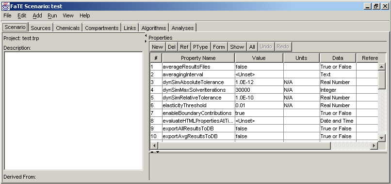
| Property Name | Description |
| appendNumberToRun | When this value is true, TRIM.FaTE appends a number (e.g., 0, 1, 2) to the end of each output file name. This option prevents the model from writing over the output files of a previous simulation within the current session. However, once the model has been shut down and restarted, TRIM.FaTE may overwrite previous output files. This property is not included in the Scenario window by default, and thus it must be added if the user wants to use a value other than the default of "true". |
| averageResultsFiles | After a FaTE Simulation has completed, TRIM.FaTE will automatically average your results files using an averaging period which you specify with the averagingInterval Property. |
| averagingInterval | An integer specifying the number of hours to average in the results files. Could also be 'monthly' or 'annual'. Although this property is always included in the scenario, the user can leave it as <Unset> if they set averageResultsFiles to "false". |
| dynSimAbsoluteTolerance | When simulateSteadyState is false, the absolute error tolerance for the differential equation solver |
| dynSimMaxSolverIterations | When simulateSteadyState is false, the maximum number of iterations the differential equation solver should use before giving up |
| dynSimRelativeTolerance | When simulateSteadyState is false, the relative error tolerance for the differential equation solver |
| elasticityThreshold | For a Sensitivity Analysis: the elasticity below which the sensitivity results should be set to 0. Elasticity is the percent change in output divided by the percent change in input. If a property has a small elasticity, it can still sometimes cause a false positive and show up as an important parameter, but the elasticity indicates how much relative change resulted from that parameter. |
| enableBoundaryContributions | When this is false, ignore the boundaryContribution properties in compartments, otherwise include them as boundary sources |
| evaluateHTMLPropertiesAtTime | The date/time at which the values of properties should be evaluated in the HTML export (MM/DD/YYYY HH:MM:SS TimeZone). Although this property is always included in the scenario, the user can leave it as <Unset> if exportHTML is set to "false". |
| exportAllResultsToDB | When this value is true, the instantaneous data files (i.e., the outputs at the output time steps) from FaTE are exported to the database (only applies if exportIngestionInputs or exportRiskECOInputs is true) |
| exportAvgResultsToDB | When this value is true, the averaged data files (i.e., the outputs at the averagingIntervals) from FaTE are exported to the database (only applies if exportIngestionInputs or exportRiskECOInputs is true) |
| exportBiotaIntakeRates | When this value is true, the intake rates for mammals and birds are placed in the MySQL database(s) generated during the run. |
| exportConcentration | When this value is true, the results are output in concentration units. |
| exportDeposition | When this value is true, the four deposition values (wet particle, dry particle, wet vapor, and dry vapor) are exported (in units of g/day/m2) to the FaTE output database. |
| exportHTML | When this value is true, the HTML export is created after the FaTE simulation has completed. |
| exportIngestionInputs | When this value is true, the inputs needed for the Expo/Ingestion module are exported to the FaTE output database. |
| exportMass | When this value is true, the results are output in mass units. |
| exportOutdoorEnvironmentBeforeRun | When this value is true, an Outdoor Environmental Export is automatically performed when a simulation is run. |
| exportPropertiesBeforeRun | When this value is true, Scenario Property Export is automatically performed when a simulation is run. |
| exportRiskECOInputs | When this value is true, the inputs needed to the Risk/Eco module are exported to the FaTE output database. |
| fateVersion | This value indicates the version of TRIM.FaTE that is currently installed on the user's computer. The value for this property is specified automatically by the model prior to performing a simulation. |
| FractionInitialConcentrations | The fraction of the initial concentrations in each compartment to be included in the simulation. |
| mySQLDataDir | The full path to the mySQL data directory (e.g., C:/mysql/data) |
| outputAdvectionFactors | If the value of this property is set to a non-empty text string, the air to air advection factors are written to a file of this name in the outputDirectory. The values in the file are in units of 1/d and are computed using the advective wind speed (m/s) * interfacial area between volume elements (m2) / volume of sending volume element (m3). |
| outputDatabaseName | Indicates the name of the MySQL output database. |
| outputDir | The directory where Simulation results should be written. |
| RiskECODatabase | Indicates the name of the Risk/Eco toxicity benchmarks database to be used when mapping FaTE biota to Risk/Eco. This name refers to the MySQL database in the root MySQL directory on the user's computer. |
| Run_ID | The Run_ID for the current simulation. This value is set automatically by the model at run time (i.e., the user does not need to specify the value). |
| significantDigits | The number of significant digits to use when writing results to a file. e.g. A value of 4 would cause results to have the form 9.999E9 |
| simulateSteadyState | Whether to perform a steady state simulation (true) or time-varying simulation (false) |
| simulationBeginDateTime | The date/time at which the simulation should begin (MM/DD/YYYY HH:MM:SS TimeZone) |
| simulationEndDateTime | The date/time at which the simulation should end, inclusive (MM/DD/YYYY HH:MM:SS TimeZone) |
| simulationStepsPerOutputStep | The number of simulation time steps in each output time step (simulation results will be output only at each output time step). To output results at each simulation time step, set this value to 1. |
| simulationTimeStep | The duration (in hours) of each simulation time step |
| steadySimAbsoluteTolerance | When simulateSteadyState is true, the absolute error tolerance for the linear equation solver |
| steadySimMaxSolverIterations | When simulateSteadyState is true, the maximum number of iterations the linear equation solver should use before giving up |
| steadySimRelaxationParam | When simulateSteadyState is true, the relaxation parameter for the Jacobi linear equation solver |
| timeZoneForResults | The time zone for which to output the simulation results |
Aside from setting the scenario properties, you need to add volume elements to your scenario (if they are not already there). This can be done by selecting "Import Volume Elements" from the File menu. You are then prompted for a file from which to import the volume elements. The format for this file is described in the Volume Element Importer Specification. During the volume element import process, the primary abiotic compartments for the volume elements are also added to the scenario (e.g., air, surface water, surface soil). NOTE: the abiotic compartments referenced in your volume elements file must be present in one of the libraries attached to the project. Be aware that volume element relationships (i.e., which volume elements are next to, above, or below other volume elements) cannot change over the course of the simulation. After the volume elements are imported, sinks are automatically created at the beginning of the simulation for the exposed faces of each volume element according to its properties (e.g., the top and bottom). The volume elements, compartments, chemicals, links, sources, and algorithms for the simulation can be edited from other tabs of the FaTE Scenario window.
To add sources to your scenario, go to the Sources View, select sources in the libraries from the right hand list and click "<< Add". If the source you want isn't shown in the list, you must add it to one of the libraries attached to the project. Refer to Table 8 for a description of any buttons on this view. The special source properties that affect the behavior of TRIM.FaTE are presented in Table 10.
|
Property Name |
Date Type |
Description |
| category | category | A hierarchical classification of the type of source (e.g., Point | Stack). |
| elevation | This is the effective elevation of the emissions source in meters. This would typically include the height of the stack above the zero elevation level for the simulation and any bouyant rise of the plume. | |
| emissionRate | The chemical-specific emission rate in grams/day. | |
| enabled | boolean | This indicates if an object is enabled for the simulation. For instance, chemicals and algorithms can be disabled. The default value is "true". |
| X | This is the X-location of the source within the modeling domain (in meters). | |
| Y | This is the Y-location of the source within the modeling domain (in meters). |
To add chemicals to the scenario, follow a similar procedure to the sources, but use the Chemicals View. Refer to Table 8 for a description of any buttons on this view. The special chemical properties that affect the behavior of TRIM.FaTE are presented in Table 11.
|
Property Name |
Date Type |
Description |
| abbreviation | string | This property is used to specify an abbreviation for a Chemical to be used in the results file. |
| CAS | string | CAS number. This property is only required if the user plans to use the TRIM.FaTE results to drive TRIM.Expo and/or TRIM.Risk. For chemicals without CAS numbers (e.g., divalent mercury), the user should refer to the relevant toxicological database (i.e., human health or ecological benchmark databases) and use the value provided in the CAS number column for the relevant chemical. |
| category | category | A hierarchical description of the type of chemical (e.g., Organic | Benzo(a)pyrene, Mercury | Elemental Mercury). A chemical's category is used in SmartLink to determine whether a link should be made by comparing its value to the value of chemicalCategory for each available algorithm. |
| doesTransform | boolean | This is a Property in the Chemical that denotes whether this Chemical transforms into another Chemical in the Scenario. The default value is "false". |
| enabled | boolean | This indicates if an object is enabled for the simulation. For instance, chemicals and algorithms can be disabled. The default value is "true". |
| reportAsOtherChemical | string | This property is used when the user wants to report the output for a given chemical as another chemical (e.g., the user might want to report the moles/mass/concentration of methyl mercury as mercury). This property is the name of the chemical that you would like to report this chemical as. This name will appear in the results file units. Must be used with reportingChemMW and molesOfReportingChemicalPerMoleOfThisChemical. |
|
reportingChemMW |
This is the molecular weight in g/mol of the chemical that you would like to report the results as. Must be used with reportAsOtherChemical and molesOfReportingChemicalPerMoleOfThisChemical. | |
| molesOfReportingChemicalPerMoleOfThisChemical | This is the number of moles of the reporting chemical in the main chemical. Must be used with reportAsOtherChemical and reportingChemMW. |
To add biotic and special abiotic compartments, use Smart Add (described below).
An example of the Compartment View is presented in Figure 5. Refer to Table 8 for a description of any additional buttons on this view. The special compartment properties that affect the behavior of TRIM.FaTE are presented in Table 12.
Figure 5. FaTE Scenario Window, Compartments View
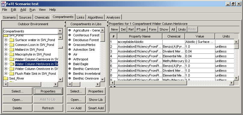
Table 12. Compartment Properties
|
Property Name |
Date Type |
Description |
| abbreviation | string | This property is used to specify an abbreviation for a Compartment to be used in the results file. |
| acceptableAbiotic | category | A hierarchical classification of the compartment (e.g., Abiotic | Air, Mammal | Meadow Vole). A compartment's category is used by the SmartAdd process to determine whether a compartment should be added to a volume element (e.g., a fish compartment can only be added to a volume element with the primary abiotic compartment with a category of "Surface water". A compartment's category is also used in SmartLink to determine whether a link should be made by comparing its value to the values of the sendingCompartmentCategory and receivingCompartmentCategory for each available algorithm. |
| boundaryContribution | boolean | This specifies a value for contribution from the boundary in g/day. If the scenario's boundaryContributionEnabled flag is 'true' and a compartment on the border of the simulation domain has this property, this property's value is the boundary contribution to the compartment. |
| category | category | A property type's category helps define the objects for which the property type could be used. For instance, a property type with category "Air" will apply to compartments with categories "Air" and "Air | Boundary Layer". If no category is specified, "All" is assumed. |
| color | string |
Color is a Volume Element property. It should be used in R,G,B format for displaying Compartments in a particular Volume Element. The R,G,B values are between 0 and 255. This color is currently only used in the Food Chain viewer to color the various Compartments. |
| concentration_g_per_kg | floating point | This property specifies the fixed concentration that should be used for a biotic compartment. Only needs to be provided if useSpecifiedConcentration is "true" for a biotic compartment. |
| concentration_g_per_L | floating point | This property specifies the fixed concentration that should be used for a surface or ground water compartment. Only needs to be provided if useSpecifiedConcentration is "true" for a surface or ground water compartment. |
| concentration_g_per_m3 | floating point | This property specifies the fixed concentration that should be used for an air, soil (surface, root, and vadose), or sediment compartment. Only needs to be provided if useSpecifiedConcentration is "true" for an air, soil (surface, root, and vadose), or sediment compartment. |
| concentrationOutputFactor | floating point | Factor used to convert the default output concentration units to some other units in the concentration output file(s). For example, this property would be set to 1000 if the default concentration units were g/m3 and the user wanted to output concentrations in mg/m3. |
| concentrationOutputUnits | string | Text string used to describe the concentration units in the concentration output file. Only needs to be provided if concentrationOutputFactor is used. |
| image | .gif, .jpg, etc file | This property links to an image file that is used in the Food Web Viewer and Transfer Factor Viewer. It is an optional property. |
| initialConcentration_g_per_kg | floating point | The initial concentration of a chemical in a compartment in grams/kg. Used for biotic compartments. |
| initialConcentration_g_per_L | floating point | The initial concentration of a chemical in a compartment in grams/liter. Used for surface and ground water compartments. |
| initialConcentration_g_per_m3 | floating point | The initial concentration of a chemical in a compartment in grams/cubic meter. Used for air, sediment, and soil (surface, root, and vadose) compartments. |
| isBiotic | boolean | This property indicates if the compartment is biotic. |
| useSpecifiedConcentration | boolean | This property indicates whether a fixed concentration should be used for a compartment. |
To add most of the links to the scenario, use Smart Link (described below), but be careful to add any additional links with "<< Link >>". Refer to Table 8 for a description of any additional buttons on this view.
Algorithms do not require a separate step, since they are added automatically to links. However, the algorithms and associated properties for each link can be viewed from this view using the Property Editor. Refer to Table 8 for a description of any buttons on this view. The special algorithm properties that affect the behavior of TRIM.FaTE are presented in Table 13.
Table 13. Algorithm Properties
|
Property Name |
Date Type |
Description |
| category | category | A hierarchical classification of the process represented by the algorithm (e.g., Ingestion | Ingestion of fish by birds) |
| chemicalCategory | category | For algorithms that do not transform chemicals, the category of chemical to which the algorithm applies. If not specified, "All" is used. |
| compartmentRelationship |
For algorithms that only apply when the compartments have a specific
relationship with one another. Allowable values are:
|
|
| doesTransformChemical | boolean | This indicates if the algorithm transforms chemicals. |
| doesTransportChemical | boolean | This indicates if the algorithm transports chemicals between compartments. |
| enabled | boolean | This indicates if an object is enabled for the simulation. For instance, chemicals and algorithms can be disabled. The default value is "true". |
| isDefaultForCategory | boolean | If multiple algorithms with the same category apply to a link, this indicates if this algorithm should be the one that is used. The default value is "true". |
| mate | string | The name of the algorithm that should be used on reciprocal links. |
| receivingChemicalName | string | For algorithms that transform chemicals, the name of the chemical on the receiving side of the link (i.e., the reactant). |
| receivingCompartmentCategory | category | The category of compartment that this algorithm can accommodate on the receiving (upstream) side of a link. |
| sendingChemicalName | string | For algorithms that transform chemicals, the name of the chemical on the sending side of the link (i.e., the reaction product). |
| sendingCompartmentCategory | category | The category of compartment that this algorithm can accommodate on the sending (downstream) side of a link. |
| transferFactor | floating-point | This is the transfer factor for an algorithm. It is almost always expressed as a formula. |
The Analyses View contains the list of sensitivity and Monte Carlo analyses for the Scenario. The dropdown menu at the top of the view allows the user to choose between Sensitivity and Monte Carlo analyses. Within the window below the dropdown menu, the user can open an existing analysis ("Open" button), create a new analysis ("New" button), rename an analysis ("Rename" button), and delete an analysis ("Delete" button). The user can also select the "Current" analysis using the "Current" button. This button allows the user to indicate which analysis should be selected when adding properties for stochastic analysis. Refer to Section 5.8 for a description of the Sensitivity Analysis tool and Section 5.9 for a description of the Monte Carlo Analysis tool.
If you find extra links, you can delete them from the Links or Algorithms
View by selecting them in the tree and clicking "Delete". If you need to make
additional links manually, from the Links View, select the compartments you
want to link on the left-hand outdoor environment panel, then select the compartment(s)
you want to link on the right-hand outdoor environment panel and click "<<
Link >>". Links will be made between the compartments selected on either
side in both directions, and any appropriate algorithms will be automatically added to the
new links. After making the manual adjustments to the links, it may be useful
to export to HTML again.
To define a time-varying property, select the property and click the "Form" button, then choose "Unevenly Time-Stepped Real Number" and click "OK." The Value Editor will appear at the bottom of the Property Editor. From the Value Editor you can either import the values from a file (e.g., for meteorological data) or enter them manually (e.g., for plant-related data that doesn't change very often). To import data from a file, click the "Import" button in the toolbar above the editor and select the file containing the data for the selected property using the File Browser that pops up. The file must be in tab-delimited text format and must have data in the forms specified in the column headings (e.g., MM/DD/YYYY for date). Once the file has been selected, click "Import." When you are finished importing or entering the data manually, click "Store" to save the data with the property (otherwise your changes will be lost).
To define a time-varying property that is to be read in from a file (a
format often used for meteorological data properties),
select the property and click the "Form" button, then choose "Unevenly Time-Stepped
Real Number From File" and click "OK.". An editor will appear at the bottom of the
Property Editor. Click the "Browse" button and use the File Browser
that pop up to select the file that contains the data for the selected
property. The file must be in the format described in Unevenly
Time-Stepped From File format. Once the file has been selected, click
"Open." Enter the data delimiter of the file in the "Delimiter" box and
click "Scan File". This will scan through the file and pick out the column
names. Select the column name that
contains your data and click the "Store" button in the toolbar above the editor.
The Select Dialog Window that appears from an outdoor environment panel has the basic options listed above, additional options to specify the type of the object (Volume Element, Compartment, Composite Compartment, or Link), and a checkbox to specify whether the object was added using the Smart Add or Smart Link feature. The latter checkbox is useful when you want to select then delete objects that were added to the outdoor environment automatically (as opposed to manually). The Select Dialogs that appear from the outdoor environment panel on the Algorithms tabs allow you to specify the category and name for the sending and receiving compartments of links. Its use for selecting other types of objects is somewhat limited.
When you are finished specifying the selection criteria, click the "Select" button to select the objects or click the "Cancel" button to cancel the selection process.
There are two types of general output from TRIM.FaTE: output data and export data. The output data are the moles, mass, and concentration outputs for each modeled chemical and time-step. These data reflect the results at the end of a time step (i.e., if a compartment has a specified concentration/mass that changes at the time of the output time step, the new value will not be shown until the following output time step). The user has the following options for the output data:
The export data contain information about the setup of a simulation, particularly the property values and relationships between compartments and volume elements. There are a number of different ways to export the information contained in TRIM.FaTE libraries and scenarios.
The Library Export Options are:
- Object Export - a text file that contains all of the information in the library; can be edited in a text editor and re-imported into TRIM.FaTE. The Object Export can be created using the "Export" command in the File menu of the FaTE Library Window.
- Property Export - a delimited text file (that can be read into Excel) that contains the complete list of properties (w/ corresponding values/formulas) in the library, i.e., the defaults for algorithm, chemical, compartment type and source properties coming into the project set-up. The Property Export can be created using the "Export" command in the File menu of the FaTE Library Window.
- Property Type Export - a delimited text file (that can be read into Excel) that contains the complete list of property types in the library. The Property Type Export can be created using the "Export" command in the File menu of the FaTE Library Window.
The Scenario Export Options are:
- HTML Export - a set of HTML files that contains a detailed description of a TRIM.FaTE scenario. It can be created before or after running a simulation, although the export following a simulation contains information not contained in an export performed prior to a simulations. This export is very useful in evaluating results because the user can see the values of formula properties and the transfer factors and fluxes between compartments. The HTML Export can be created using the "Export" command in the File menu of the FaTE Scenario Window or by setting the "exportHTML" and "evaluateHTMLPropertiesAtTime" properties in the Scenario View.
- Link Export - a text file that contains a list of all of the links and their associated algorithms in a scenario. The Link Export can be created using the "Export" command in the File menu of the FaTE Scenario Window.
- Outdoor Environment Export - a delimited text file (that can be read into Excel) that contains the list of volume elements, compartments and links defined for the project scenario, along with the algorithms associated with each link. The Outdoor Environment Export can be created using the "Export" command in the File menu of the FaTE Scenario Window.
- Property Export - a delimited text file (that can be read into Excel) that contains the customization of the library for the scenario, including any geographic variation in property values/formulas across the scenario compartments. It also includes the link, scenario (e.g., start time and end time of run, export options), sink, and volume element properties that have been defined in the project scenario. The Property Export can be created using the "Export" command in the File menu of the FaTE Scenario Window.
Boundary conditions are used to account for the chemical mass that is transported into the system from outside the modeling domain. Thus, they should only be added to compartments that are on the exterior of the modeling domain (i.e., they have at least one face that is not neighbored by any other volume element). NOTE: The current version of the model only supports adding boundary conditions to air compartments.
To specify a boundary concentration,
- Add the property boundaryContribution to the compartment(s). The default value of this property is:
boundaryContribution(containingVolumeElement.chemical.boundaryConcentration_g_per_m3, containingVolumeElement.horizontalWindSpeed, containingVolumeElement.windDirection)
Therefore, by default, the information regarding the boundary contribution is taken from the volume element in which the compartment resides.
- Add the property boundaryConcentration_g_per_m3 for the appropriate chemical to the compartment's volume element and set it to the appropriate concentration.
There are two properties in each compartment that affect the units in which the results are written to the concentration output file(s):
- concentrationOutputFactor
- concentrationOutputUnits
By default, the concentrationOutputFactor is set to 1.0 and the concentrationOutputUnits are set to the default concentration units for that compartment. The default concentrations units for each type of compartment are:
- g/m3 for air, sediment, and soil (surface, root, and vadose) [calculated by dividing the chemical mass in the compartment by the volume of the volume element containing the compartment];
- g/L for surface water and ground water [calculated by dividing the chemical mass in the compartment by the volume of the volume element containing the compartment]; and
- g/kg wet weight for biota [calculated by dividing the chemical mass in the compartment by the total wet weight of the compartment.
However, the user may change this by inputting a factor (which may be a constant or a formula) and changing the name of the units to correspond with the units after the factor is applied.
For example, if the user wanted to write soil compartment concentration (default = g/m3 wet) as g/g dry weight, the user would:
- Change the value of the concentrationOutputFactor property to the following formula:
1.0 / (Comparment.rho * Compartment.VolumeFraction_Solid * 1000)
- Set the concentrationOutputUnits property to "g/g dry weight"
The concentrations for the selected soil compartments would then be in "g/g dry weight".
The currently available TRIM.FaTE libraries use the default concentrationOutputFactor and concentrationOutputUnits for all compartments except the three soil compartments and the sediment compartment. The soil and sediment compartments have modified with the appropriate factors to output concentrations in units of "g/g dry weight".
There are times when the user may wish to report a simulated chemical as another. For example, risk analysts may wish to see the mass of Methyl Mercury reported as Mercury. To do this, you must add three properties to the chemical whose output you would like to change.
1. reportAsOtherChemical - This is the name of the other chemical that you would like to report this chemical as. This name will appear in the results file units. This might read "Hg" in the above example of Mercury.
2. reportingChemMW - This is the molecular weight in g/mol of the chemical that you would like to report as. This would be 201.0 in the case of Mercury.
3. molesOfReportingChemicalPerMoleOfThisChemical - This is the number of moles of the reporting chemical in the main chemical. In the case of Mercury in Methyl Mercury, this is 1.
There are three primary properties used in specifying initial concentrations: initialConcentrion_[units], initialConcentration_[units]_UserSupplied, and FractionInitialConcentrations. The property initialConcentrion_[units]_UserSupplied is a Compartment Property that contains the value for the initial concentration the user wants to use for a particular compartment. The property FractionInitialConcentrations is a Scenario Property that specifies the fraction of initialConcentrion_[units]_UserSupplied that should be used in the simulation (e.g., 0 if the user did not want to include initial concentrations for a particular simulation, 1 if the user wanted to use all of the user-specified initial concentrations in a simulation). The property initialConcentrion_[units] contains a formula that calculates the initial concentration that the model that will be used in the simulation by multiplying initialConcentrion_[units]_UserSupplied by FractionInitialConcentrations.
The details for setting up initial concentration are provided below.
- Add one of the pairs of properties to the compartment(s) for the desired chemical(s):*
- initialConcentration_g_per_m3 and initialConcentration_g_per_m3_UserSupplied (for all abiotic media except surface and ground water)**,
- initialConcentration_g_per_L and initialConcentration_g_per_L_UserSupplied (for surface and ground water), or
- initialConcentration_g_per_kg and initialConcentration_g_per_kg_UserSupplied (for biota).
- Input your initial concentrations for each chemical using the initialConcentration_[units]_UserSupplied property.
- Set the initialConcentrations_[units] property to the appropriate formula (if the property was already added, it should be set to the correct formula):
- containingScenario.FractionInitialConcentrations * compartment.Chemical.initialConcentration_g_per_m3_UserSupplied (for all abiotic media except surface and ground water)
- containingScenario.FractionInitialConcentrations * compartment.Chemical.initialConcentration_g_per_L_UserSupplied (for surface and ground water), or
- containingScenario.FractionInitialConcentrations * compartment.Chemical.initialConcentration_g_per_kg_UserSupplied (for biota).
- OPTIONAL. If you would like to scale the initial concentrations by a particular fraction, or turn them off all together, adjust the scenario property "FractionInitialConcentrations" accordingly. The default value for the property is 1.0. Some example uses of the property:
- If you would like to turn off the initial concentrations, set FractionInitialConcentrations to 0.0.
- If you would like to set the initial concentrations to 50% of their original values (as set in step (2)), set FractionInitialConcentrations to 0.5.
- If you would like to use the initial concentrations as set in step (2), set FractionInitialConcentrations to 1.0.
* Be sure to check if the properties are already added for the compartment(s) in which you want to set initial concentrations. In most cases, the properties should already be there.
** Although the initialConcentration units for soil and sediment are grams per m3, the output units for both media in the available libraries are grams per gram (dry weight). The model will likely be modified in the future to allow the user to input initial concentrations in the same units as the output concentrations, but this functionality is not currently available.
To specify that the concentration for a compartment remain fixed throughout the simulation:
- Add the property useSpecifiedConcentration to the compartment(s) and set it to "true". This property should not have any Chemical associated with it (i.e., select "none" when prompted for chemical).
- Add one of the following properties (with a Chemical) and set the value to the appropriate concentration level:
- concentration_g_per_m3 (for all abiotic media except surface and ground water),
- concentration_g_per_L (for surface and ground water), or
- concentration_g_per_kg (for biota).
If more than one of the concentration_[units] properties is added, they will all be ignored.
Note: If you want the value at the first time step to be the same as the fixed value, you must also specify the initial Concentration.
To specify an abbreviation for a Compartment or Chemical to be used in the results file, add a Property called abbreviation.
Sources, when first created, do not have any properties for emissions because it is not possible to know which chemical(s) it should be emitting. So, prior to running a simulation, you should add an emissionRate property for each of the chemicals emitted by each source. Based on the location information given for the source, the system will determine the volume element to which the source emits. If the emissionRate is constant, the "Form" of the property should be "Constant Real Number". If the emissionRate varies with time, the "Form" of the property should be either "Unevenly Time Stepped Real Number" or "Unevenly Time Stepped Real Number from File". If the emissionRate is a function, the "Form" of the property should be "Formula Real Number".
5.5.8 Specifying Output File Names and Directories
TRIM.FaTE creates output files using the name of the scenario, the names of the modeled chemicals, the type of output (moles, mass, or concentration), and a internally-generated ID (e.g., A0). For example, the elemental mercury concentration file for a scenario named "TestCase" might be "TestCase_Elemental_Mercury_concA1.txt". If multiple runs of the same scenario are performed during a single session (i.e., without closing the scenario or project), the model will name these files using different IDs, thus eliminating the potential for overwriting existing output files. However, if multiple runs of a scenario are performed during separate sessions (i.e., closing the scenario between runs), the model could assign an ID that corresponds to the ID of an existing output file, and thus the user could accidentally overwrite existing output files. To prevent this, the user should always check the output directory prior to performing a simulation to make sure there are no existing output files with the same scenario name in the output directory. If there are, the user may be best served by changing the output directory of the current run (this is done by changing the outputDir property in the list of scenario properties under the Scenario View).
You may start TRIM.FaTE with a set of command line options that allow you to run a specific FaTE Scenario. To use this feature:
- Add either "-run" or "-runthenexit" after the TRIM.FaTE startup command in the batch file you use to run TRIM.FaTE. "-run" will open TRIM.FaTE, run the selected simulation, and leave TRIM.FaTE open after the simulation completes. "-runthenexit" will open TRIM.FaTE, run the selected simulation, and then exit TRIM.FaTE.
- Add "-showGUI true[or false]" to specify whether to show the TRIM.FaTE GUI during the run.
- Add "-verify true [or false]" to specify whether to verify the scenario.
- Add "-prefs" and the name of a preferences file to specify the user preferences.
- Add "-project" and the name of the Project file that you wish to run.
- Add "-fatescenario" and the name of the Scenario within the Project that you wish to run.
- Add "-propsfile" and the name of a property file to run a simulation overriding the selected properties in the scenario
Example:
%JRE% -Xmx400m -classpath [.....] java gov.epa.trim.main.Main -run -showGUI true -project c:\TRIM\models\woodland.trp - fatescenario forest -propsfile FullMaine_properties.txt
NOTE: Currently, running in batch mode only works for deterministic simulations and not for Monte Carlo or sensitivity runs.
When importing the volume element file, you will be prompted to provide information about the map projection of the volume element layout. There are four basic items that should be specified (in the following order):
- Projection Family - The projection family is selected first from the drop-down menu labeled "Available Projection Families". The current version of the model includes:
- Lambert
- Latitude-Longitude, and
- Universal Transverse Mercator (UTM).
- Ellipsoid - The ellipsoid is selected next from the drop-down menu labeled "Ellipsoids". The current version of the model includes:
- Sphere
- WGS 1994
- Clarke 1880
- International 1909
- SGS 1985
- GRS 1967
- GRS 1980
- WGS 1960
- WGS 1966
- WGS 1972
- Name - This is an optional items that can be filled in by the user to name the projection.
- Parameters - The parameter values that must be completed depend on the selected projection family. For Lambert projections, the user must specify:
- Secant Latitude South
- Secant Latitude North
- Central Longitude
- Central Latitude
For Latitude-Longitude projections, the user must specify Central Longitude.
For UTM projections, the user must specify the UTM Zone.
TRIM.FaTE can be run in two modes: dynamic and steady-state. For a dynamic run, you should simply follow the instructions provided in Section 5.2, using whatever input data you determine is appropriate, and making sure that the Scenario Property "simulateSteadyState" is set to "false". Performing a steady-state run is identical, except for the following:
- Set the Scenario Property "simulateSteadyState" to "true".
- No time-varying data (e.g., meteorological data) can be included in the steady-state simulation. If you are setting up a steady-state simulation from a dynamic simulation, you should replace all of the time-varying data with constants (possibly averages of the time-varying data for some properties).
- All links FROM groundwater compartments must be disabled by setting the "enabled" property to "false". This step is required because the transfers from ground water are so slow that they act as virtual sinks and prevent the solver from finding a steady-state solution.
- In some cases, using time keywords in formulas (e.g., time.hour) can slow down the simulation. For instance, using the hour will force calculations to be performed for each hour in the day, whereas they might actually otherwise need to be calculated only once per day or even less frequently.
- When adding a new chemical, be sure to set the doesTransform property to the appropriate value. For example, doesTransform would be set to "true" for elemental mercury and "false" for benzo(a)pyrene.
The various tree views can be used to view which Compartments are contained in which Volume Element and which links go into and out of which Compartment. But it may be easier to view some relationships graphically.
If you want to view the diet of a certain animal (this only applies to biotic Compartments) select the Compartment on the Compartments View and go to the View menu and select Food Chain. This will bring up a window that will display the food chain leading to that Compartment with the percentage diet on each link. An arrow is drawn if there is a Link between two Compartments and there is an active algorithm on that Link. The value that is placed on the link is related to a Property in the predator that starts with "fractiondiet" and ends with the name of the prey. An example of the food chain window is provided in Figure 6.
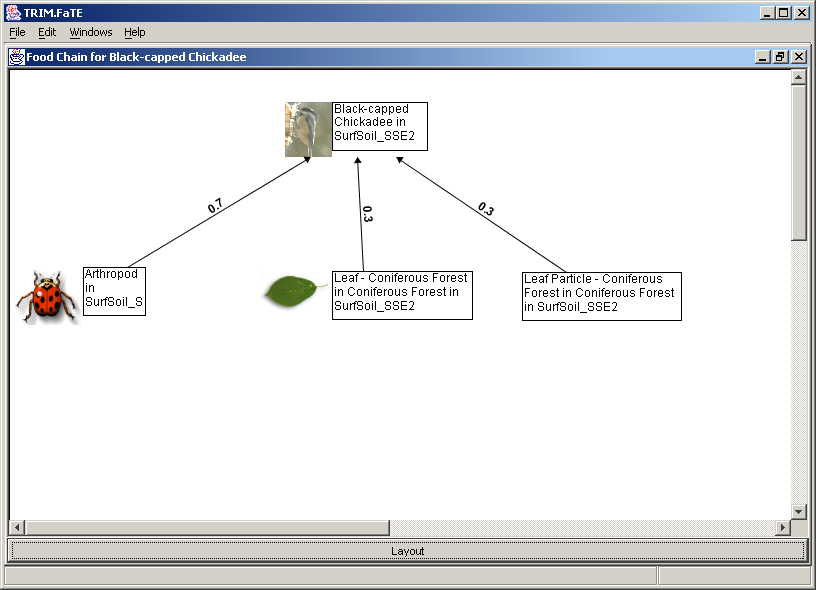
You can associate images with certain Compartments to make the food chain easier to view. To do this, add a Property called "image" to each Compartment and set it's value to be the path to an image file that matches the Compartment.
After completing a simulation, you can view the results in several ways. TRIM.FaTE contains a text file viewer as well as a graphical display of the results. Note that for large simulations with a large number of Compartments or a large number of time steps, it may be best to average the results before attempting to view them.
If your Compartment names are very long and you would like to use an abbreviation, you can add a Property called "abbreviation" that will use the abbreviation as the column name in the results files.
To view the results in a table, go to the View menu and select Run Results. This will present a window that will allow you to choose the Chemical and the units that you wish to view. You may also choose between the Basic Viewer and the Analysis Engine table viewer. Note that the analysis engine table has been under active development through 2006, but the basic viewer has not been updated since 2003. Make your selections and then press OK. This will bring up a results file for the last TRIM.FaTE simulation that you performed (you must have performed at least one simulation to view results.) To view the results from an earlier run, you can press the Browse button and select the file yourself. This will bring the file into a tool called JART (Java Analysis and Reporting Tool). It contains many sorting and filtering options to allow you to analyze and organize your output results. This tool is documented here.
After completing a simulation, you may also view the results graphically from a "bird's eye" view. Click the Analysis Tab and press the Show Results button. This will bring up a file browser. Select the results file that you wish to view and press Open. Note: you can only view simulation results for the currently open FaTE Scenario. An example of the Graphical Results Viewer is provided in Figure 7.
Figure 7. Graphical TRIM.FaTE Results
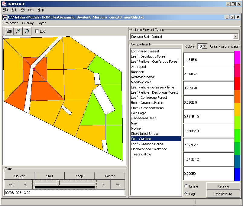
On the left is a view of the Volume Elements looking down from above. If a Compartment is displayed, you will be able to see it's concentration based on the color legend on the right. The type of Compartment that is displayed is selected in the Compartments list in the middle of the screen. The legend for the colors and values is displayed on the right and the time step is displayed below the plot. The units of the currently displayed Compartment are displayed above the legend.
The Compartments in TRIM.FaTE are laid out in Volume Element at different levels. It would not be easy to view two Compartments that were in Volume Elements that are on top of each other. In order to prevent this type of conflict, you can only view Compartments that are in one type of Volume Element at a time. Within those Volume Elements, you can view one type of Compartment that they contain at a time. In the above picture, the "Surface Water" Volume Elements are selected. There are two of these and they are represented by the red and orange polygons in the display. The Compartments list is filled with the types of Compartments that are found in the Surface Water Volume Element and the values for the Common Loon are currently being viewed. To view Compartment in a different type of Volume Element (Air, Groundwater, Surface Soil...), select a different value from the Volume Element Types list and select the Compartment type that you wish to view from the Compartments list. To print out the current plot, you can press the print button (with the printer icon) to the upper left of the plot. You can also use the magnifying glasses to zoom in and out. If you would like to see the Lat/Lon and X/Y coordinates of certain points in the plot, check the Location check box and move your mouse to the point. The values will be displayed next to the check box.
The legend for the colors and values is on the right hand side. When you select a new Compartment, TRIM.FaTE will automatically rescale the legend based on the minimum and maximum values for the Compartment that you are viewing. The scale can be set to linear or logarithmic by selecting the Linear or Log radio buttons below the list of values. At the top is a drop down box where you can select the number of colors that you want to use. This can range from 2 to 20. If you would like to change the colors, you can click on the color and change it. After this, you should press Redraw to redraw your plot with the new colors. You can also change the values by hand and use the Redraw button to reflect these changes. You can also enter a minimum value in the lowest text field and a high value in the topmost text field and press the Redistribute button to redistribute the between the minimum and maximum value that you added.
The time step that is being displayed can be controlled from the Time panel beneath the plot. To advance the time step forward, press the ">" button. To move the time step backward, press the "<" button. The "<<" button will set the plot to the first time step and the ">>" will set it to the last time step. You can also move the slider to change the time step. Note that for very large files, there may be a delay between when you move the slider and when the plot refreshes. The plot will also animate forward in time. You can press the Start button to begin the animation and use the Stop button to stop at the current time step. The Faster and Slower buttons will speed up or slow down the animation. TIP: Always try to "rewind" to the beginning of the time period before changing compartment types. This simple step will greatly decrease the time it takes to bring up the data for the newly selected compartment type.
You can add GIS layers on top of the TRIM.FaTE data results by going to the Layer menu and selecting Edit Layers. This will bring up a dialog that will contain information about the layers in your plot (an example is provided in Figure 8). The first layer is the parcel layer. This is the outline of the parcels in your Scenario. The next layer is the data layer. This contains the colored polygons that represent the data you are currently displaying.
Figure 8. Layer Control Window
To add a layer, press the Add button. This will bring up an open file dialog and allow you to choose a file to add. Currently, TRIM.FaTE can only read ESRI shape files. To show a layer, check the Show check box next to it's name. To hide a layer, uncheck the Show check box. You can raise and lower layers by selecting them and using the Raise and Lower buttons. A layer can be deleted from the plot by selecting it and pressing the Delete button. To set options for the layer, like polygon and line colors, press the Options button on the same row as the layer name.
The layer options window (shown in Figure 9) allows you to change attributes of the polygons, line and points in the layers. For a polygon, you can specify whether it is filled or open by using the Filled and Outline radio buttons on the right. If you select Outline, then only the Outline color will be used to draw the outline of the polygon. If you select Filled, then the Fill color will be used to fill the polygon and the Outline color will be used to draw outline of the polygon. You can change the color by clicking on the color box. Note that you can set the transparency of the color to allow lower layers to bleed through higher layers. The line thickness of the outline in pixels can be set using the Thickness box. Lines can be edited using the options in the Lines area. If there are Points in the shape file, the type, color and size can be set in the Points area. The available types are circle, square, triangle, diamond, cross and star. If you would like to preview the changes before you close the window, you can press Apply to apply the changes. Press OK to close and apply the changes.
Figure 9. Layer Options Window
Figure 10 provides an example of GIS layers displayed with TRIM.FaTE data. Some of the streams and ponds in the area have been loaded and their color has been set to a transparent blue to allow the data colors to be seen with the water boundaries.
Figure 10. GIS Layers on top of TRIM.FaTE data
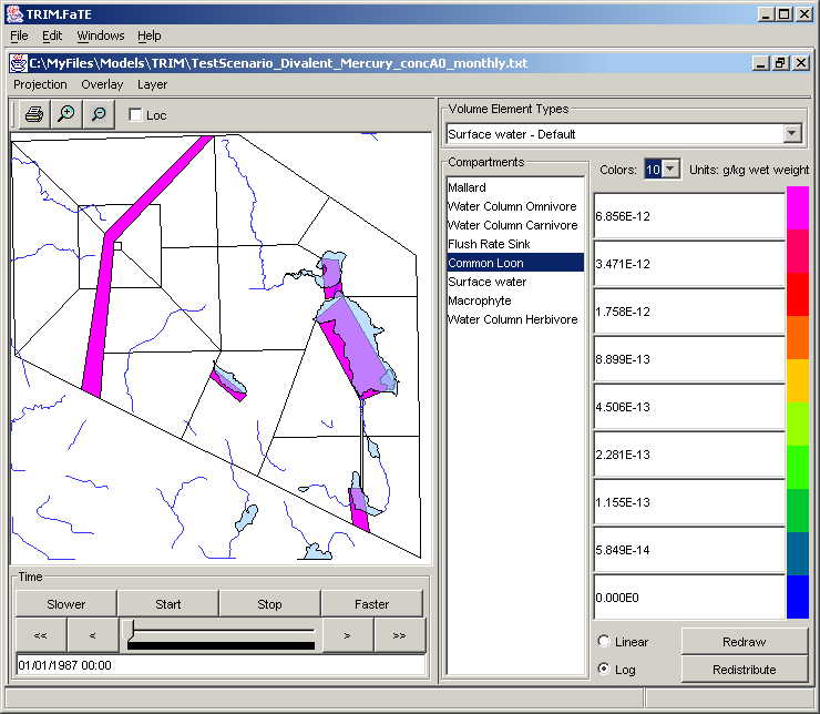
You can also add your own overlays to the map with points, lines and polygons (as demonstrated in Figure 11). These are specified in a text file format which is detailed here. With this format, you can place labeled points and polygons on your plots to provide context for the data. Polygons may be either filled or unfilled and you can specify the fill color, line color, line thickness and line style. For labeled points, you can specify the symbol type, color and size. You can also specify the font color, type, style, size and orientation about the point. This feature could be used to add cities, buildings, park outlines and roads to the plot. Below is an example of some of features of the overlay file.
Figure 11. Overlay of points on data
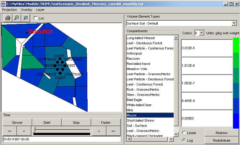
Before running a sequence of simulations, the user should make certain that the scenario is set up correctly. It is advised that you set the output directory property in the scenario to identify the location where the run results will be written.
The first step in performing a sequence of simulations is to configure the runs. To do this, open the Sequential Runs Window (Run -> Sequential Runs). This will bring up a window similar to Figure 12. By default, there will be one run, named "Run 1" in the Runs pane. You can add new runs and duplicate, delete, or open existing runs using the buttons below the Runs pane. You can also rename a run using the Run -> Rename menu item.
The second step in performing a sequence of simulations is to select the properties and objects that will be varied for each run (all other object properties in the scenario will be the same for all of the sequential runs). This step involves the following tasks:
After selecting all of the properties that you want to vary in the sequential runs, go through each of the runs and change the properties values to the values you want to use in each of the simulations. Finally, select the simulations you want in the Runs pane of the Sequential Runs Window and select "All Selected Runs" from the Run menu.
Figure 12. Sequential Run Window
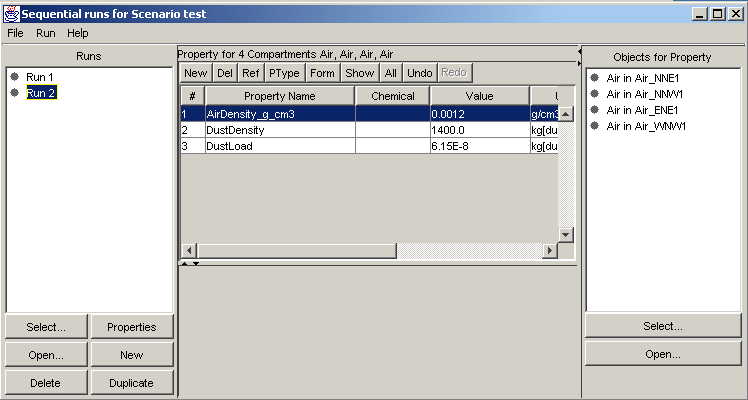
The TRIM.FaTE sensitivity analysis functionality is accessed via the Analyses view of the Scenario window by selecting Sensitivity Analyses from the drop-down box in the upper left corner. The window below the drop-down box (i.e., the Sensitivity Analyses pane) lists the sensitivity analyses that are in the current scenario. By default, an empty sensitivity analysis is created with every scenario and is labeled with the name of the scenario. To add a new sensitivity analysis, click the New button and enter a name when prompted. The other buttons below the analyses window can be used to delete, rename, or open analyses. In the example shown in Figure 13, five sensitivity analyses have been created.
To view specific information about an analysis, the user can bring up the Sensitivity Analysis window. This window is opened by selecting a sensitivity analysis name and clicking the Open button or by double-clicking the analysis name in the Sensitivity Analyses listing. Alternatively, the user can access this window by clicking on the Run pull-down menu in the scenario window, selecting Sensitivity Analysis, and then selecting the appropriate analysis in the dialog box that appears. The Sensitivity Analysis Window contains tabs that access three views:
The features associated with each of these views is described in more detail in the sections that follow.
Figure 13. FaTE Scenario Analysis View
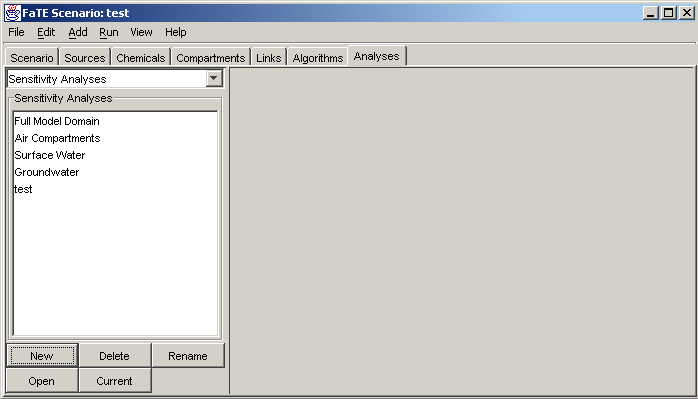
There is no default set of properties for a TRIM.FaTE sensitivity analysis.
To designate the properties that will be varied, the user must add properties to
the sensitivity analysis from the scenario window. The following steps describe
this process.
To view the properties that have been added to an analysis, open the Sensitivity Analysis window and click the Properties tab. Next, select the property (or properties) of interest. When you select the property (or properties), the objects associated with these properties will be displayed in the Objects for Property pane. An example is provided in Figure 14.
Figure 14. Sensitivity Analysis Window, Properties View
Once the appropriate properties have been added to the analysis, the new values to be included in the sensitivity analysis runs can be set via the Properties view. As shown in Figure 14, each property is listed on a separate row of the table that appears on the left side of this view, with values for the following data fields in the columns (note that not all of these columns are visible in the window presented in Figure 14; the horizontal scroll bar at the bottom of the window can be used to view the hidden columns):
The objects to which the currently selected properties apply (e.g., compartments, links, chemicals) will appear in the pane on the right under the label Objects for [object name(s)], where the name(s) in the brackets will be filled in depending on which properties are currently highlighted in the table.
The precise new value for a property can be set directly or by specifying a percentage change from the base value. To set the value directly, the user can edit the value displayed in the Value column for that property in the Sensitivity Analysis window. Alternatively, the value can be changed by a percentage of the original value by selecting the property, entering a percent variation in the text box at the top of the Properties view, and clicking the Adjust button. A positive percent variation will increase the value (a positive sign (+) is not required). Negative numbers can be entered using the negative sign () to denote a decrease in the value. Note that the actual percent should be entered in this window (e.g., to increase the values by 10 percent, enter 10, not 0.10). A different percent variation can be used for different properties, or the same percent variation can be implemented for multiple properties by selecting multiple properties (using the shift or control key) and entering a value for variation.
When adjusting property values by a given percent for a sensitivity run, the values are always adjusted from the original base case value. For example, if property values are initially varied by 10 percent, and the variation is then changed to 20 percent, the new values will vary by 20 percent of the original base case values, not by 20 percent of the 10 percent varied values. If desired, the user can reset one (or all) Property values to their original base case values by selecting the property (or all properties) and clicking the Reset button.
Information about the status and location of the simulation runs that are being performed is summarized on the Runs View within the Sensitivity Analysis window (see Figure 15). In the table that appears on this view, information about individual runs is presented on separate rows, including:
Note that the table on the Runs View is simply used to present information to the user (i.e., the user cannot modify this table directly to change run information).
Two important options must be set by the user via the Runs view:
Figure 15. Sensitivity Analysis Window, Runs View
Once these options have been set, the model simulations associated with the sensitivity analysis can be run. Note that a separate simulation is completed for the base case and each of the runs (i.e., one for each of the properties that is selected to be varied). To execute these simulations, select one or more run in the table on the Runs View and click the Run Selected button at the bottom of the view. This will start the selected runs as a batch. While the simulations are processing, a small window with a Stop button will appear that can be used to stop the batch of simulations at any point during the run (it may take a minute or two for the simulation to stop after the button is clicked).
After the simulation for a given run has been completed, the status of that run in the table on the Runs View will change to Successful, Warnings, or Failed. An output subdirectory will be created within the main output directory (specified above) for each run as listed in the Subdirectory column. For each run included in the analysis (i.e., the base case run plus each of the runs for the properties that were perturbed), a complete set of output files will be saved in the corresponding subdirectory. These simulation results are used by TRIM.FaTE to calculate quantitative sensitivity results, as described in the following section.
Important Note: Depending on the complexity of the scenario and, likely, whether the model is run in dynamic or steady state mode, including a large number of runs in a single batch may cause model execution problems. Running multiple batches of runs (each containing a subset of the runs comprising a sensitivity analysis) may reduce the potential for this problem.
After the simulations for the base run and the perturbed properties have been completed, the sensitivity calculations to be completed using the simulation results can be specified via the Analysis View within the Sensitivity Analysis window (see Figure 16). To obtain sensitivity results, the user selects compartments and chemicals for which to evaluate the sensitivity of the properties that were varied from their base values. The steps involved in specifying and executing the calculations are described below.
Figure 16. Sensitivity Analysis Window, Analysis View
Note that Steps 2 and 3 are not required if the sensitivity simulations are run in steady-state mode. If the simulation is being run in steady-state mode, TRIM.FaTE will automatically shade the date and averaging interval windows and the user will not be able to access them.
With the completion of the analysis step, TRIM.FaTE creates a sensitivity summary file for each combination of chemical (per user specification in step 5) and form of results (per user specification in the Runs view).
To perform additional sets of sensitivity calculations from the same set of sensitivity runs (e.g., to generate sensitivity analysis results for other combinations of compartments and chemicals, or to evaluate the sensitivity at a different date/time by entering a different date/time in Step 2), Steps 2 through 6 can be repeated. Note, however, that TRIM.FaTE will not change the name of the output file(s). That is, existing summary results files will be overwritten if Steps 2 through 6 are repeated for the same TRIM.FaTE sensitivity analysis. Therefore, if additional calculations are to be performed to produce new summary files, the user should first rename the previous summary files in order to preserve them.
For sensitivity calculations on results from dynamic TRIM.FaTE simulations, Steps 2 and 3 specify which results (i.e., from which time point or, for averaged results, which time interval) to use in the sensitivity calculations. The Average Interval input provides a way for the user to use time-averaged results rather than an instantaneous point in time. For example, if the Average Interval is specified as annual and the user enters a date/time that falls within the 20th year of the simulation, then the annual average of the simulation results for the 20th year will be used to calculate that set of sensitivity results. The user should note that the sensitivity score value that is calculated by TRIM.FaTE could vary depending on the averaging interval used and the selected time.
Summary Files
TRIM.FaTE generates summary results for the sensitivity analysis based on the user specifications listed in the previous section. These summary results will be saved to a series of text files in a subdirectory of the output directory specified in the Runs view of the Sensitivity Analysis window. The subdirectory will be named Sensitivity Analysis and will include an additional subdirectory with the name of the analysis.
One summary file will be created for each combination of chemical and form of results (i.e., mass, moles and/or concentration). Each row within a given summary file contains sensitivity results for a property that was perturbed and a selected compartment for which the output was of interest (i.e., the compartments listed in the Selected Compartments pane). For example, if four properties were varied in the sensitivity analysis, and three compartments were selected on the Analysis view, the sensitivity results file for a selected chemical and form of results (e.g., moles of divalent mercury) would contain 12 rows of data. Each row in the summary results file will include, in separate columns, values for the sensitivity parameters generated by TRIM.FaTE as presented in Table 15. Key measures of sensitivity are highlighted in boldface in Table 15. Note that the calculation of the sensitivity score relies on the coefficient of variation provided by the user for each perturbed property in the TRIM.FaTE statistics file.
Sensitivity analysis summary results files will be semicolon delimited and can be opened in a spreadsheet program. Alternatively, they can be viewed within a TRIM.FaTE window by clicking the View Results button at the bottom of the Results view screen. A new TRIM.FaTE window will appear that contains an array of results for the current compartment(s) and chemical(s) (i.e., the compartment(s) and chemical(s) selected on the Analysis view).
Table 15. Sensitivity Output File Columns
| Column Title | Description |
|
Property |
The name of the property that was varied. |
|
Chemical |
The chemical for the property that was varied, if appropriate. |
|
ObjectType |
The type of object in which the property was varied (e.g., compartment, link, chemical) |
|
ObjectName |
The name of the object for which the property was varied. |
|
CV |
The coefficient of variation for this property (as provided in the statistics file). |
| VE_Info | The volume element name (e.g., SW_lake), if the object named in the previous column is a volume element or compartment, or the name of the link, if the object named in the previous column is a link (e.g., from Soil - Surface, to Surface water from SurfSoil_SE2 to SW_lake). If the object is a chemical, algorithm, or source, this column will be blank. |
| NumObjs | The number of objects for which the property was varied (e.g., if the property being varied is a property of three surface water bodies, this column would read 3). The name of the first volume element appears in the VE_Info column. |
|
Initial_Input |
The initial input for the property value in the base case. |
|
Perturbed_Input |
The input value of the property after perturbation for the sensitivity analysis. |
|
%deltaInput |
The percent change in the input value between the base run and the perturbed run. |
|
Initial_Output |
The initial output value (i.e., base case) in the compartment of interest. |
|
Perturbed_Output |
The perturbed output value in the compartment of interest. |
|
%deltaOutput |
The percent change in the output value in the compartment of interest. |
|
Sensitivity |
The sensitivity is the ratio of the change in the output value (relative to the base case) to the perturbation of the input value. |
|
Elasticity |
The elasticity is a measure of the sensitivity relative to the initial values that were used and is calculated by the formula (deltaOutput / InitialOutput) / (deltaInput / InitialInput). |
|
Score |
The sensitivity score is the elasticity weighted by a normalized measure of the variability of the parameter and is calculated by the formula Elasticity * CV (where the CV is expressed as a fraction, not a percentage). |
|
Absolute Score |
The absolute score is the absolute value of the Sensitivity Score. |
Individual Sensitivity Run Files
The run results from which the sensitivity measures are calculated consist of model results files for each unique combination of modeled chemical, form of results (i.e., moles, mass, or concentration), and perturbed property value. The format of these files is identical to the format of the outputs from a deterministic simulation. These results files are saved in subdirectories of the analysis results folder that are named using the property names included in the analysis. For example, using the output directory specified in Figure 15, the results for the runs in which the DustLoad property was perturbed will be saved in the following directory:
c:\MyFiles\ModelsTRIM\data\Public Reference\test\SensitivityAnalysis\test\ DustLoad3
Note that TRIM.FaTE assigns a subdirectory name for the individual run results that matches the name of the property being varied in the analysis with the addition of a numeral. The numeral corresponds to the order in which the property was selected for the analysis, starting with zero and skipping one (i.e., 0, 2, 3, 4...). This number is used to differentiate the subdirectory with these run results from the subdirectory with results corresponding to a different run involving the same property names. Thus, the numeral 3 was attached to the folder name by TRIM.FaTE to differentiate these results from separate runs related to the same property name (e.g., if the property DustLoad for a different compartment was added to the analysis).
A Monte Carlo analysis involves running several simulations and varying a specified group of Properties in each simulation. These properties might have been chosen by selecting the most influential input Properties from a Sensitivity Analysis or based on some other criteria. Unlike the Sensitivity Analysis where properties are varied by a percentage of the base value, the selected properties in a Monte Carlo analysis are varied by sampling from the input distributions of the properties, which are defined in a statistics file which you provide.
To access the Monte Carlo feature, go to the Analyses view within a TRIM.FaTE scenario and select Monte Carlo Analyses from the drop-down box in the upper left corner (see Figure 13). The window below the drop-down box (labeled the Monte Carlo Analyses pane) will list the Monte Carlo analyses that are in the current scenario. By default, an empty Monte Carlo analysis is created with every scenario and labeled with the scenario name. To add a new Monte Carlo analysis, click the New button and enter a name when prompted. The other buttons below the Analyses window can be used to delete, rename, or open analyses.
To view specific information about an analysis, the user can bring up the Monte Carlo Analysis window. This window is opened by selecting a Monte Carlo analysis name and clicking the Open button or by double-clicking the analysis name in the Monte Carlo Analyses pane. (Alternatively, the user can access this window by clicking on the Run pull-down menu in the scenario window, selecting Monte Carlo Analysis, and then selecting the desired analysis in the dialog box that appears.) Like the Sensitivity Analysis Window, the Monte Carlo Analysis Window contains tabs that allow the user to access three views:
Each of these views is described in more detail in the sections that follow.
The process for selecting properties to be included in the Monte Carlo analysis (i.e., properties for which values will be varied according to a specified distribution) is nearly identical to the process used to add properties to the sensitivity analysis (see Section 5.9.1). The steps to be followed are described here.
To view the properties that have been added to an analysis, click on the Properties tab within the Monte Carlo analysis window. The properties selected for inclusion in the Monte Carlo analysis will be listed in the left-hand window along with the original property values that were assigned for the simulation. The objects to which these properties apply will be shown in the right-hand window. An example of the Properties view within the Monte Carlo Analysis window for a sample analysis entitled test is presented in Figure 17. In this example, three properties have been added to the current analysis. The highlighted property in the example (AirDensity_g_cm3) has been added for the five air compartments shown in the right-hand object window.
To set up a separate Monte Carlo analysis, designate a different run as Current as described in Step 1, and repeat Steps 2 through 6 until all of the desired properties have been added to the run. Properties can be removed from an analysis by highlighting the unwanted property and clicking the Del button above the properties table.
Figure 17. Monte Carlo Analysis Window, Properties View
The Properties view is also used to specify where the model can find the statistical distribution data for the selected properties. These data are stored in the statistics file for the scenario (which can be the same file in which the coefficients of variation for the sensitivity analysis are stored). Refer to the Statistics File Format document for information on how to set up and format the statistics data file. The user should specify the location of the statistics file using the Statistics File window at the top of the Properties view (see Figure 17). The file name and directory can be entered directly by the user (by clicking in the window and typing the directory and name of the file), or the user can click the ... button to bring up a file browser that allows the user to find and select the appropriate file.
In addition, the directory where the Monte Carlo analysis output will be saved is also specified on the Properties view in the Output Directory window. Note that this procedure is slightly different from setting the output directory for the sensitivity analysis (when it is specified via the Runs view).
Information about the status and location of the Monte Carlo analysis model runs that will be performed is summarized on the Runs view (see Figure 18). The user defines three analysis settings on this view.
Figure 18. Monte Carlo Analysis Window, Runs View
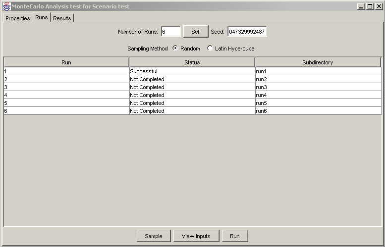 =
=
After following these steps, the user must click the Sample button at the bottom of the view to sample from the distributions for each property. If one of the Properties does not exist in the statistics file, TRIM.FaTE will notify the user via an error message, and the user must edit the statistics file and resave the file to the location specified on the Properties view. The property values assigned by TRIM.FaTE for the Monte Carlo analysis can be viewed by clicking the View Inputs button at the bottom of the view (the values will appear in a new TRIM.FaTE window).
To start running the simulations for the Monte Carlo analysis, the user should select the runs to be performed by highlighting them in the table and clicking the Run button at the bottom of the view. A small window containing a Stop button will appear; this button can be clicked to abort the batch of runs.
Important Note: Depending on the complexity of the scenario and, likely, whether the model is run in dynamic or steady state mode, including a large number of runs in a single batch may cause model execution problems. Running multiple batches of runs (each containing a subset of the runs comprising a Monte Carlo analysis) may reduce the potential for this problem.
After the simulations for the Monte Carlo analysis have been completed, the results can be collated (i.e., combined to a single summary file) via the Results view (see Figure 19). The following six steps should be completed to collate the results.
Figure 19. Monte Carlo Analysis Window, Results View
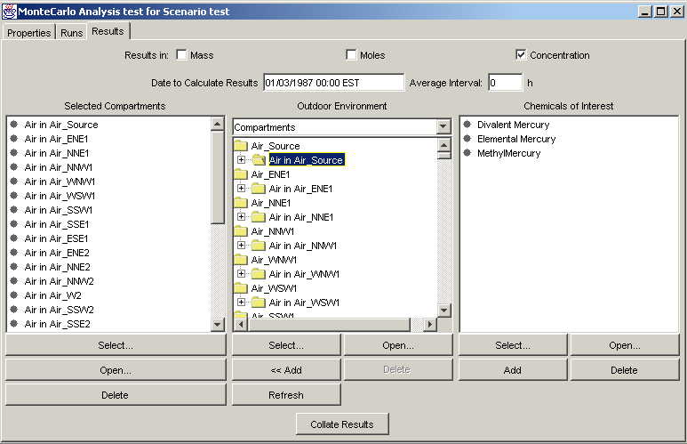
Note that Steps 2 and 3 are not required if the sensitivity simulations are run in steady-state mode. If the simulation is being run in steady-state mode, TRIM.FaTE will automatically shade the date and averaging interval windows and the user will not be able to access them.
Once the results have been collated by TRIM.FaTE, there will be one results file for each combination of chemical and form of results. For example, if mass and concentration are both selected as the form of results and three chemicals are included in the simulations, six results files will be generated. Each results file that is created will contain an array of results, with results for each user-specified compartment saved in the columns of the array and the results for each run saved in the rows in the array.
To complete a Monte Carlo analysis for the same set of properties (i.e., to collate files at a different date/time by entering a different date/time in Step 2), Steps 2 through 6 can be repeated. Note, however, that TRIM.FaTE will not change the name of the output file(s). That is, existing collated results files will be overwritten if Steps 2 through 6 are repeated for the same TRIM.FaTE Monte Carlo analysis. Therefore, if additional calculations are to be performed to produce new collated results files, the user should first rename the previous results files in order to preserve them.
For collating Monte Carlo results from dynamic TRIM.FaTE simulations, Steps 2 and 3 specify which results (i.e., from which time point or, for averaged results, which time interval) to use in collating the Monte Carlo results. The Average Interval input provides a way for the user to use time-averaged results rather than an instantaneous point in time.
Each collated results file will be saved in a subdirectory of the output directory specified on the Properties view of the Monte Carlo analysis window (see Figure 17). The subdirectory will be named MonteCarlo and will include an additional subdirectory with the name of the analysis. The model results for individual runs will also be saved in folders within the scenario name subdirectory of the MonteCarlo subdirectory according to the names specified on the Runs view. A collated Monte Carlo results file can be used to calculate statistics on the outputs of the Monte Carlo simulations (e.g., mean or median values in the compartments of interest; percentiles). TRIM.FaTE does not calculate such statistics internally; they must be calculated off-line by the user.
Several tools have been developed to assist users in processing TRIM.FaTE input and output data. A brief description, as well as a link to a more detailed description, of each tool is provided below.
Simulation
Import/Export and Files
Formulas
General
If you haven't used TRIM.FaTE since version 1.3, you should also check out the New Features in Version 2.0. The features added in Version 2.5 are:
If you haven't used TRIM.FaTE since version 2.5, you should also check out the New Features in Version 2.5. The features added in Version 2.6 are:
If you haven't used TRIM.FaTE since version 2.6, you should also check out the New Features in Version 2.6. The features added in Version 3.0 are:
New Features in Version 3.4 (12/22/2003)
The new features in Version 3.4 are:New Features in Version 3.5 (11/12/2004)
The new features in Version 3.5 are:New Features in Version 3.6 (10/14/2005)
The new features and issues addressed in Version 3.6 are:Volume Element Importer Specification
Compartment Chooser File Format
Java Analysis and Reporting Tool (JART) Documentation
Last updated October 14, 2005