Executive Summary
The Clean Air Status and Trends Network (CASTNET) measures atmospheric pollution concentrations across the United States and Canada. The primary purpose of the network is to provide data to evaluate the effectiveness of national and regional air pollution control programs. CASTNET ozone measurements are used to gauge compliance with National Ambient Air Quality Standards. CASTNET data are also used to provide input to the National Atmospheric Deposition Program’s Total Deposition Hybrid Method for estimating total deposition and for regional air quality model evaluation. This report presents 2013 maps of ozone levels and sulfur and nitrogen pollutant concentrations and estimates of deposition fluxes, and it examines trends in air quality since 1990. CASTNET measured ozone levels from 82 analyzers operated at 80 locations in 2013 and rural, regionally representative concentrations of sulfur and nitrogen species at 92 monitoring stations in 90 locations.
Key Results and Highlights through 2013
- The mean fourth highest daily maximum 8-hour average ozone (O3) concentration for 2013 at eastern reference sites was 63 parts per billion (ppb) or, equivalently, 0.063 parts per million (ppm), the lowest in the history of the network. At the western reference sites, the value was 68 ppb. Exceedances of the 8-hour National Ambient Air Quality Standard of 0.075 ppm were measured at eight sites (four eastern and four western) during the most recent three-year period (2011 through 2013).
- Mean annual sulfur dioxide (SO2) and particulate sulfate (SO42-) concentrations measured at eastern CASTNET reference sites have declined significantly over the 24-year period 1990 through 2013 and showed a substantive reduction since 2005. The 2013 mean SO2 concentration of 1.4 micrograms per cubic meter (µg/m 3 ) of air was the lowest value over the history of the network. Three-year mean annual SO2 levels declined 80 percent while SO42- concentrations declined 59 percent at eastern reference sites from 1990 through 2013. Three-year mean SO2 concentrations declined by 54 percent, and SO42- levels dropped by 20 percent at western reference sites over the 18 year period (1996 through 2013). Figure E-1 and Table E-1 summarize the long-term changes in measured pollutant concentrations.
- The 80 percent reduction in SO2 concentrations between 1990–1992 and 2011–2013 at CASTNET eastern reference sites is consistent with the steep reduction in electric generating unit SO2 emissions (84 percent) from states in the East.
- Three-year mean annual total (dry + wet) sulfur (S) deposition (Table E-2) estimated for the eastern reference sites declined by 66 percent from 1990–1992 through 2011–2013. Total S deposition estimates aggregated over western reference sites fell by 39 percent from 1996–1998 through 2011–2013.
- Three-year mean annual concentrations of total nitrate (NO3-), which is comprised of nitric acid (HNO3) plus particulate NO3-, declined 41 percent at eastern sites over the 24 year period. Three-year mean annual total NO3- levels measured at western reference sites dropped by 27 percent over the 18-year period. Three-year mean annual concentrations of particulate ammonium (NH4+) decreased 50 percent at eastern sites and 17 percent at western sites over the same periods.
- The 41 percent reduction in total nitrate concentrations measured at the 34 eastern reference sites between 1990–1992 and 2011–2013 did not correspond to the reduction in oxides of nitrogen (NOx) emissions (78 percent) as closely as SO2 concentrations tracked SO2 emissions because, in addition to power plants, transportation and other combustion sources produce NOx emissions and contribute to total NO3- concentrations.
- Estimates of 3-year mean total nitrogen (N) deposition (dry + wet) fell by 24 percent from 1990 through 2013 at eastern reference sites. Total N deposition estimated for western reference sites declined by 18 percent over the 18 years.
- Air quality monitors were operated continuously at eight sites across the United States to measure trace-level pollutant concentrations. Concentrations of total reactive oxides of nitrogen (NOy) were measured at all eight sites, SO2 at three sites, and carbon monoxide at two sites. NOy concentrations were highest at suburban sites, e.g., Beltsville, MD in the Washington, DC area, and lowest at the high-elevation, mountainous sites, e.g., Pinedale, WY.
- Measurements from 2013 and historical data collected over the period 1990 through 2012 were analyzed relative to data quality indicators and their numerical measures, e.g., for precision, accuracy, completeness, bias, and comparability. The results of these analyses, which are discussed throughout the report, demonstrate that CASTNET continues to produce information of the highest quality, and CASTNET data can be used with confidence.
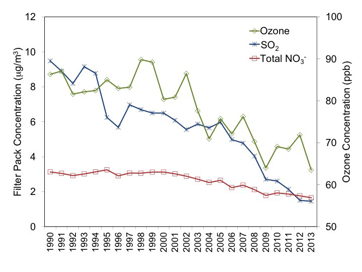
Table E-1 Trends in Aggregated Western and Eastern Sulfur and Nitrogen Pollutant Concentrations
| Pollutant (µg/m 3) | Western Sites | Eastern Sites | Percent Changed | |||
|---|---|---|---|---|---|---|
| 1996-98 | 2011-13 | 1990-92 | 2011-13 | West | East | |
| SO2 | 0.6 | 0.3 | 8.9 | 1.7 | -54 | -80 |
| SO42- | 0.8 | 0.6 | 5.4 | 2.2 | -20 | -59 |
| Total NO3- | 1.0 | 0.7 | 3.0 | 1.8 | -27 | -41 |
| NH4+ | 0.3 | 0.2 | 1.8 | 0.9 | -17 | -50 |
Table E-2 Trends in Aggregated Western and Eastern Sulfur and Nitrogen Pollutant Deposition Estimates
| Pollutant (kg/ha/yr) | Western Sites | Eastern Sites | Percent Changed | |||
|---|---|---|---|---|---|---|
| 1996-98 | 2011-13 | 1990-92 | 2011-13 | West | East | |
| Dry S | 0.3 | 0.2 | 5.1 | 1.1 | -40 | -78 |
| Total S | 1.3 | 0.8 | 12.9 | 4.3 | -39 | -66 |
| Dry N | 0.9 | 0.6 | 2.2 | 1.1 | -35 | -51 |
| Total N | 2.5 | 2.1 | 7.5 | 5.7 | -18 | -24 |
Chapter 1: CASTNET Overview
The Clean Air Status and Trends Network (CASTNET) is a nationwide air quality monitoring network that began operation in 1991. Its principal function is to provide air pollutant concentration data to evaluate the effectiveness of national and regional emission control programs and to determine compliance with ozone National Ambient Air Quality Standards. CASTNET was also designed to determine trends in rural atmospheric ozone, nitrogen, and sulfur concentrations and deposition fluxes of nitrogen and sulfur pollutants. CASTNET data are used to provide input to the National Atmospheric Deposition Program’s Total Deposition Hybrid Method and for regional air quality model evaluation. CASTNET is managed and operated by the U.S. Environmental Protection Agency in cooperation with the National Park Service and other federal, state, and local partners. CASTNET was established under the 1990 Clean Air Act Amendments, expanding the National Dry Deposition Network, which began in 1987. In 2013, CASTNET operated 92 monitoring stations throughout the contiguous United States, Alaska, and Canada. The network’s measurements demonstrate the continuing reductions in ozone, nitrogen, and sulfur pollutant concentrations, which have declined significantly over the last 24 years.
Background
The U.S. Congress established the Acid Rain Program (ARP) under Title IV of the 1990 Clean Air Act Amendments (CAAA). The ARP was enacted to reduce emissions of sulfur dioxide (SO2) and nitrogen oxides (NOx) from electric generating units (EGUs), and it has produced significant reductions in emissions since 1995. Since then, other air pollution control programs have been instituted to reduce emissions of SO2 and NOx. For example, the Clean Air Interstate Rule (CAIR) was enacted in 2005 to reduce emissions in 27 eastern states and the District of Columbia. This rule created three separate trading programs: an annual NOx program, an ozone (O3) season NOx program, and an annual SO2 program. The CAIR O3 seasonal and annual NOx programs began in 2009 while the CAIR annual SO2 program began in 2010. Emission control programs are summarized in Table 1-1. The emission reductions achieved under these programs have resulted in a dramatic improvement in air quality as demonstrated by air pollutant concentrations measured by CASTNET and other cooperating networks. By 2013, EGUs required to comply with ARP/CAIR had reduced their SO2 emissions to about 3.2 million tons and NOx emissions to about 1.7 million tons, decreases of 84 and 78 percent, respectively, from 1990 levels.
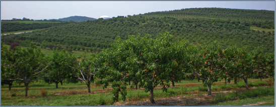
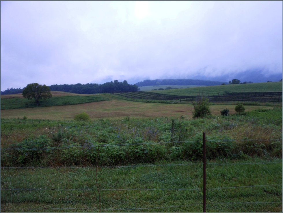
Scenic view from Arendtsville, PA (ARE128)
Table 1-1 Major SO2 and NO2 Emission Control Programs Established Since 1990
| Ozone Transport Commission (OTC) |
| Established under the 1990 CAAA, this commission consists of states primarily located in the Northeast and Mid Atlantic regions. The OTC developed the OTC NOx Budget Program, which operated from 1999 to 2002. As part of this program, 11 states and the District of Columbia entered into a memorandum of understanding to achieve regional emission reductions of NOx through the use of control technologies and an O3 season cap and trade program. |
| NOx State Implementation Plan (SIP) Call |
| Issued in 1998 to reduce the regional transport of ground-level O3, the NOx SIP Call required states to reduce O3 season NOx emissions by meeting emission budgets. |
| NOx Budget Trading Program (NBP) |
| This market-based cap and trade program was developed under the NOx SIP Call and replaced the OTC NOx Budget Program in 2003. The NBP was created to reduce NOx emissions from power plants and other large combustion sources in 20 eastern states and the District of Columbia. It operated from 2003 to 2008. |
| Clear Air Interstate Rule (CAIR) |
| Promulgated in 2005, CAIR was designed to reduce emissions of SO2 and NOx in 27 eastern states and the District of Columbia, and it replaced the NBP in 2009. This rule created three separate trading programs: an annual NOx program, an O3 season NOx program, and an annual SO2 program. In December 2008, CAIR was remanded but remained in place until January 1, 2015 when the Cross-State Air Pollution Rule became effective (EPA, 2014d). |
| Cross-State Air Pollution Rule (CSAPR) |
| On July 6, 2011, CSAPR was promulgated to require 28 states in the eastern half of the United States to significantly improve air quality by reducing power plant emissions that cross state lines and contribute to ground-level O3 and fine particle (PM2.5) pollution in other states. The rule was scheduled to replace CAIR starting in 2012 and was designed to reduce annual SO2, annual NOx, and O3 season NOx emissions while providing sources with flexibility in how to comply with the program. CSAPR Phase 1 implementation began January 2015. The callout later in this chapter summarizes the status of CSAPR. |
Congress also mandated in the 1990 CAAA that the U.S. Environmental Protection Agency (EPA) provide consistent, long-term measurements for determining relationships between changes in emissions and subsequent changes in air quality, atmospheric deposition, and ecological effects. The network operated 92 monitoring stations in 2013 throughout the contiguous United States, Alaska, and Canada. CASTNET is sponsored by EPA and the National Park Service (NPS), which began its participation in 1994 and operated 26 sites in 2013. The Bureau of Land Management (BLM) began participation in CASTNET in late 2012 and now operates five sites in Wyoming.
In 2013, a new site was added by BLM at Fortification Creek, WY (FOR605) and by NPS at Dinosaur National Monument, UT (DIN431). Additionally, trace-level gas monitoring for nitrogen oxide/total reactive oxides of nitrogen was established at Pinedale, WY (PND165); Rocky Mountain National Park, CO (ROM206); and Cranberry, NC (PNF126). In 2013, eight CASTNET sites performed trace-level gas monitoring. The site at Mount Rainier, WA (MOR409) was discontinued in 2013.
This report summarizes CASTNET monitoring activities and the resulting concentration and deposition data collected over the 24-year period from 1990 through 2013. Additional information, previous annual reports, other CASTNET documents, and the CASTNET database can be found on the EPA website. The website provides a complete archive of concentration and deposition data for all EPA- and NPS-sponsored CASTNET sites.
Cooperating Networks
CASTNET monitors air quality and deposition in cooperation with other national and international networks. EPA uses CASTNET and these other long-term national networks to assess the effectiveness of emission control programs.
National Atmospheric Deposition Program (NADP) operates:
- National Trends Network (NTN), which includes about 260 monitoring stations with wet deposition samplers to measure the concentrations and deposition rates of air pollutants removed from the atmosphere by precipitation. NTN operates wet deposition samplers at or near virtually every CASTNET site.
- Ammonia Monitoring Network (AMoN), which operates passive ammonia (NH3) samplers at about 40 CASTNET locations. AMoN, in operation since 2007, provides information on 2 week average NH3 concentrations.
- Mercury Deposition Network (MDN), which operates samplers to measure mercury (Hg) in precipitation. MDN samplers are operated at several CASTNET sites.
- Atmospheric Mercury Network (AMNet), which measures atmospheric concentrations of gaseous oxidized, particulate-bound, and elemental Hg at about 18 locations in the continental United States, Canada, Hawaii, and Taiwan in order to estimate dry and total Hg deposition.
See NADP’s website for detailed information on each of these sub-networks.
Canadian Air and Precipitation Monitoring Network (CAPMoN) operates 30 measurement sites throughout Canada and one in the United States. CASTNET and CAPMoN both operate filter pack samplers in Ontario, Canada. CAPMoN operates a wet deposition sampler at the Pennsylvania State University CASTNET site (PSU106, PA).
EPA’s National Core Monitoring (NCore) reports on particulate matter (PM) mass; PM species; O3, SO2, nitrogen oxide/total reactive oxides of nitrogen (NO/NOy), and carbon monoxide (CO) concentrations; and meteorological parameters at approximately 80 sites.
BLM’s Wyoming Air Resources Monitoring System (WARMS) operates eight sites and the meteorological system at one of the EPA-sponsored CASTNET sites (PND165) in Wyoming. Five of the WARMS sites are CASTNET-protocol sites.
Interagency Monitoring of Protected Visual Environments (IMPROVE) measures speciated aerosol pollutants that affect visibility near more than 20 CASTNET sites. For more information, see IMPROVE.
Locations of Monitoring Sites
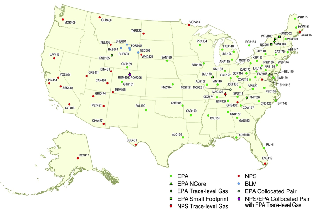
The locations of the CASTNET monitoring sites that were operational during 2013 are depicted in Figure 1 1. Ninety-two monitoring sites were operated at 90 distinct locations. To estimate precision across the network, collocated sites were operated at Mackville, KY (MCK131/231) and Rocky Mountain National Park, CO (ROM406/206) during 2013. The ROM406/206 pair ensures consistency between the two agencies sponsoring the most sites. EPA operates ROM206, and NPS operates ROM406. Of the two Rocky Mountain monitoring sites, ROM406 is considered the regulatory monitoring site for O3. Appendix A provides the location of each site by state and includes information on start date, latitude, longitude, elevation, identification of nearby NADP site, land use, terrain type, operating agency, and if the site is a reference site used for trends. Two new sites (DIN431, UT; FOR605, WY) were added to the network during 2013.
Supreme Court Upholds Cross-State Air Pollution Rule (CSAPR)
On July 6, 2011, CSAPR was promulgated under the Clean Air Act’s Section 110 “Good Neighbor” Provision. This rule requires 28 states in the eastern half of the United States to improve air quality by reducing power plant emissions of SO2 and NOx. These pollutants react in the atmosphere to form fine particles and ground-level O3 and are transported long distances, making it difficult for downwind areas to achieve the National Ambient Air Quality Standards (NAAQS).
CSAPR replaces EPA's 2005 Clean Air Interstate Rule (CAIR). A December 2008 court decision kept the requirements of CAIR in place temporarily but directed EPA to issue a new rule to implement Clean Air Act requirements concerning the transport of air pollution across state boundaries. CSAPR responds to the court's concerns.
According to analysis at the time of promulgation, with CSAPR in place, most of the counties with monitors in the region covered by CSAPR are projected to meet the 1997 and 2008 O3 and 2006 PM2.5 NAAQS. CSAPR will provide cleaner air and healthier lives for Americans by improving air quality in counties in the eastern, central, and southern United States.
The timing of CSAPR's implementation has been affected by a number of court actions. On December 30, 2011, CSAPR was stayed prior to implementation. On April 29, 2014, the U.S. Supreme Court issued an opinion reversing an August 21, 2012 D.C. Circuit decision that had vacated CSAPR. Following the remand of the case to the D.C. Circuit, EPA requested that the court lift the CSAPR stay and toll the CSAPR compliance deadlines by three years. On October 23, 2014, the D.C. Circuit granted EPA's request. Accordingly, CSAPR compliance started on January 1, 2015, and Phase 2 compliance begins in 2017.
Figure 1-1 CASTNET Sites Operational during 2013
Prince Edward, VA (PED108)
Measurements Recorded at CASTNET Sites
In brief, the network operates 92 sites at 90 locations. All CASTNET sites measure weekly ambient concentrations of acidic pollutants, base cations, and chloride (Cl -) using a 3-stage filter pack with a controlled flow rate (AMEC, 2012; 2013c). Gaseous pollutant measurements include SO2 and nitric acid (HNO3). Particulate concentrations include sulfate (SO4 2-), nitrate (NO3 -), ammonium (NH4 +), magnesium, calcium, potassium, sodium, and Cl -. The filter pack is exchanged each Tuesday and shipped to the analytical chemistry laboratory for analysis. Ambient temperature is measured at 9-meters (m) at all sites in part to support conversion of concentrations to local conditions.
Most CASTNET sites also include a temperature-controlled shelter and continuous O3 monitoring system. The O3 inlet and filter pack are located atop a 10-m tower. Some CASTNET sites also measure trace-level SO2, CO, and NO/NOy. In 2013, meteorological parameters were measured at 6 EPA-, 25 NPS-, and 4 BLM-sponsored CASTNET sites. Measured meteorological parameters include 2-m temperature, wind speed and direction, standard deviation of the wind direction, solar radiation, relative humidity, precipitation, and surface wetness. Meteorological measurements were discontinued in 2010 at most EPA-sponsored CASTNET sites.
Quality Assurance Program
The CASTNET Quality Assurance (QA) program was designed to ensure that all reported data are of known and documented quality in order to meet CASTNET objectives. The QA program was developed to ensure intra-network consistency and comparability and to deliver data that are reproducible and comparable with data from other monitoring networks and laboratories. The 2013 QA program elements are documented in the CASTNET Quality Assurance Project Plan (QAPP; AMEC, 2012; 2013c). The QAPP includes standards and policies for all components of project operation, from site selection through final data reporting, with appendices that provide standard operating procedures (SOPs) for CASTNET operations.
Data quality indicators (DQI) such as precision, accuracy, and completeness are used to assess CASTNET measurements and supporting activities. Routine assessment and analysis help guarantee the production of high-quality data and information to meet project objectives. Measurements taken during 2013 and historical data collected over the period 1990 through 2012 were analyzed relative to DQI and their associated metrics. Results from these analyses are available in quarterly and annual QA reports posted on the EPA CASTNET website. S. Selected analyses are summarized in callout boxes labeled, “QA Program Summary,” where appropriate throughout this report.
Estimating Dry, Wet, and Total Deposition
Total deposition was assessed using the NADP’s Total Deposition Hybrid Method (EPA, 2014f; Schwede and Lear, 2014), which is a hybrid approach that combines data from established ambient monitoring networks and large scale models. To estimate dry deposition, ambient measurement data from CASTNET and other networks were merged with dry deposition rates and flux output from the Community Multiscale Air Quality (CMAQ) modeling system. Wet deposition estimates were made from precipitation chemistry measurements and precipitation amounts from the Parameter-elevation Regressions on Independent Slopes Model (PRISM). Dry and wet deposition fluxes were added to obtain the estimates of total deposition that are discussed in Chapter 5.
Scenic view from Speedwell, TN (SPD111)
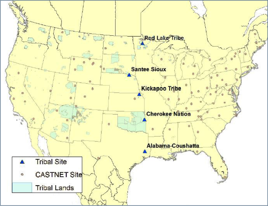
Building Tribal Partnerships with CASTNET Monitoring Sites
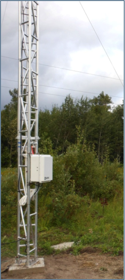
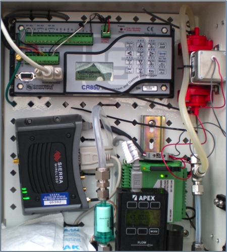
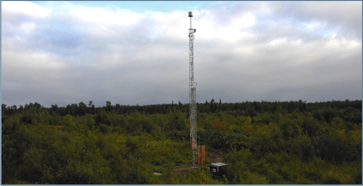
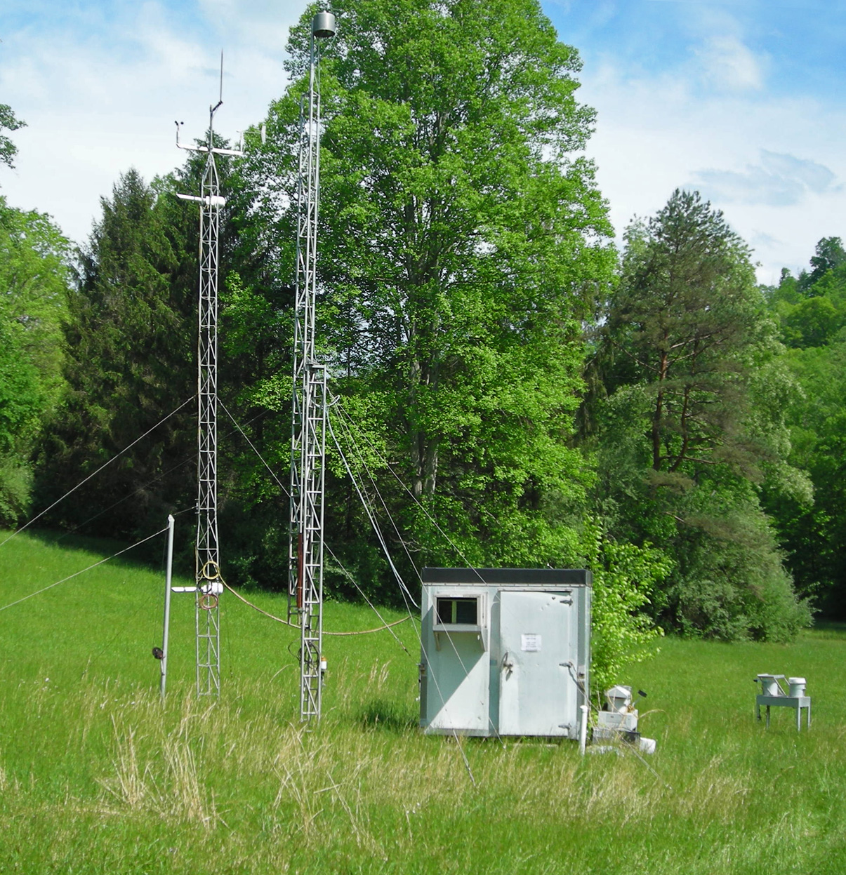
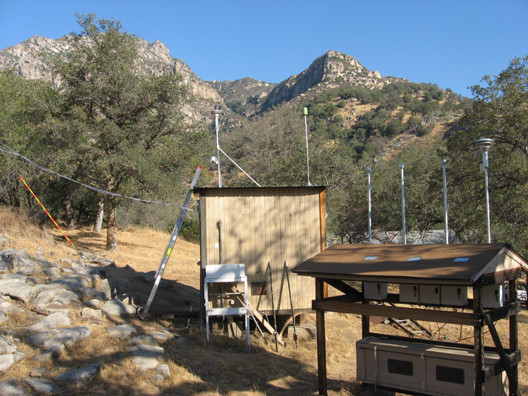
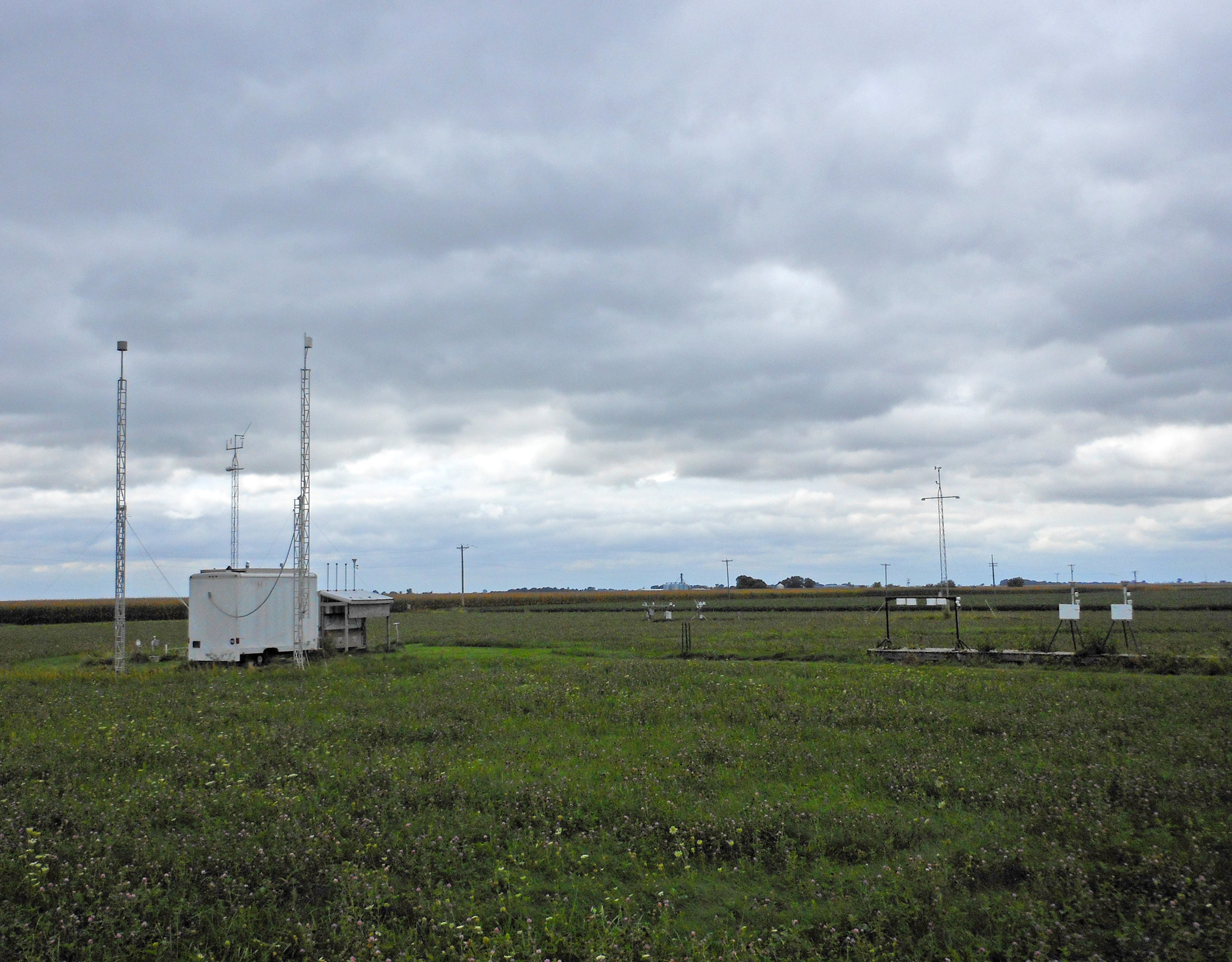
EPA partners with Cherokee Nation, OK (2002); the Alabama-Coushatta Tribe, TX (2004); and the Santee Sioux Tribe, NE (2006) to operate CASTNET sites on tribal lands. These tribes have been a part of CASTNET since the years noted in parentheses. In 2012, CASTNET developed a small-footprint monitoring station that does not require a temperature-controlled shelter. The new type of monitoring station includes a 10-m sampling tower, 3-stage filter pack, pump, flow meter, data logger, and cellular modem (Figure 1-a). Two other tribes have entered into partnerships with EPA with the advent of the small-footprint monitoring station. The Kickapoo Tribe in Kansas and the Red Lake Band of Chippewa Indians in Minnesota agreed to operate small-footprint sites. The Kickapoo Tribe site (KIC003, KS) was established in February 2014 in Powhattan, Kansas. The Red Lake, MN site (RED004) shown in Figure 1-a began in August 2014. The Kickapoo Tribe and the Red Lake Band partnered with CASTNET to build upon their existing environmental monitoring programs.
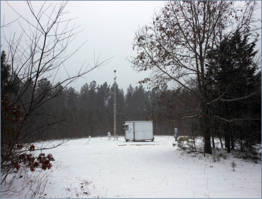
Figure 1-a Small Footprint Site Operated at Red Lake, MN (RED004)
The operation of CASTNET monitoring sites on tribal lands provides benefits to the tribes and EPA. The CASTNET measurements contribute data on atmospheric pollutant and deposition impacts to areas important to tribes and provide information that can be used to determine:
- Negative effects to land and water quality, and
- Health effects due to O3 and/or PM2.5 formation
The measurements help the tribes understand the effects of prescribed burns, wild fires, and nearby point or urban sources. The CASTNET sites at Cherokee Nation in Oklahoma and Kickapoo Tribe in Kansas are located near middle schools, and students have access to the monitoring sites, equipment, and data, thereby enhancing science/environmental education. The tribal personnel assigned to operate the monitors are trained and become trainers. For example, EPA provided training to Cherokee Nation in 2002, and Cherokee Nation has since provided training to many tribal partners.
For EPA, partnerships are important for operating a consistent, stable, long-term monitoring network. Current tribal sites fill in gaps in the network within the central United States (Figure 1-b), and tribes provide much needed support for operations and infrastructure. Many sites operate collocated monitoring instruments on behalf of NCore, NADP, MDN, AMNet, and AMoN. The Cherokee, Alabama-Coushatta, and Santee Sioux tribal sites provide data to AIRNow and EPA’s Air Quality System (AQS).
EPA will continue its outreach efforts to existing tribal partners and other interested tribes in upcoming years. CASTNET will develop tools for viewing data, reporting on air quality and deposition fluxes in tribal regions, training, and preparing “frequently asked questions” for tribal air-monitoring groups.
Chapter 2: Ozone Concentrations
CASTNET is the principal network for monitoring rural, ground-level ozone concentrations in the United States and providing critical information on geographic patterns in rural ozone levels. Ozone data measured at EPA-sponsored sites from 2011 through 2013 were submitted to EPA’s Air Quality System and were evaluated with respect to the current National Ambient Air Quality Standards (EPA, 2008a). Maps of fourth highest daily maximum 8-hour average (DM8A) ozone concentrations for 2013 and 3-year averages of fourth highest DM8A ozone concentrations for 2011 through 2013 and for 2000 through 2002 are provided. Trends in fourth highest DM8A ozone concentrations for eastern and western reference sites are presented.
Most CASTNET sites operate an O3 analyzer that measures hourly average concentrations, which are archived in the CASTNET database and delivered to AQS. During 2013, 82 O3 analyzers operated at 80 sites throughout the network. Data from these sites, with the exception of Howland, ME (HOW191) and the collocated sites at Yosemite National Park, CA (YOS204) and ROM206, CO, which are designated as non-regulatory, are used to calculate design values as three years of Title 40 Code of Federal Regulations (CFR) Part 58-compliant data become available. CASTNET’s geographic coverage of the United States provides data that are essential for evaluating rural O3 concentrations in the context of the O3 NAAQS and in terms of presenting information on trends and geographic patterns in regional O3.
A design value is a statistic that describes the air quality status of a given area relative to the level of the NAAQS. Design values change as each new 3-year database of monitored ozone concentrations becomes available. Design values are used to classify nonattainment areas, assess progress towards meeting the NAAQS, and develop control strategies to achieve the NAAQS. For example, if 3-year averages of 2011–2013 fourth highest DM8A ozone concentrations are used for purposes of attainment designation and exceed 0.075 parts per million (ppm), then ozone concentrations will have to be reduced to 0.075 ppm or below, to achieve the current ozone NAAQS.
The information presented in this chapter includes maps and trends in the annual fourth highest DM8A O3 concentrations measured at CASTNET sites. Additional maps of O3 concentrations can be viewed at from the NPS Air Atlas.
Measurements from 34 CASTNET eastern and 17 western reference sites (see Appendix A) were analyzed to determine trends in O3 concentrations. The reference sites were also used to show trends in ambient nitrogen and sulfur concentrations (Chapter 4). The 34 eastern sites have been reporting CASTNET measurements since at least 1990 and the 17 western sites since at least 1996.
National Ambient Air Quality Standards for Ozone
Current Standards
| Ozone 1 | Primary Standard | Secondary Standard | |
|---|---|---|---|
|
Level |
Averaging Time |
Level |
Averaging Time |
|
0.075 ppm |
8-hour 1 |
0.075 ppm |
8-hour 1 |
The primary O3 NAAQS is designed to protect public health. The secondary standard is designed to protect public welfare and the environment. Both O3 NAAQS are set at a level of 0.075 ppm averaged over eight hours for the annual fourth highest value.
On November 25, 2014, EPA proposed to update both the primary and secondary standards for O3. Both standards would be 8-hour standards set within a range of 0.065 to 0.070 ppm. EPA (2014c) has requested comments on the proposed standards as well as comments on (1) reducing the NAAQS to 0.060 ppm or (2) retaining the existing standard. The proposed 8-hour secondary standard of 0.065 to 0.070 ppm is equivalent, based on the W126 index, to a level of protection of 13 to 17 ppm-hour averaged over three years (EPA, 2014b). The W126 index is a seasonal measure often used to assess the impact of O3 exposure on ecosystems and vegetation. W126 values for the period 2011 through 2013 and for 2013 are presented in a separate callout at the end of this chapter (pp. 16-17).
Note: 1To attain this standard, the 3-year average of the fourth highest DM8A O3 concentrations measured at each monitor within a specified area must not exceed 0.075 ppm or 75 parts per billion (ppb) in practice (effective May 27, 2008; EPA, 2008a). O3 concentrations are commonly presented in units of ppb.
EPA and other federal, tribal, state, and local agencies measure O3 concentrations on an hourly basis through national and local monitoring programs. AMEC followed EPA procedures (1998) to estimate O3 design values and 2013 fourth highest DM8A O3 concentrations at CASTNET sites, including measurements affected by exceptional events. “Exceptional events are unusual or naturally occurring events that can affect air quality but are not reasonably controllable using techniques that state, tribal, or local air agencies may implement in order to attain and maintain the NAAQS” (EPA, 2013). CASTNET O3 data are used to gauge compliance with the NAAQS at EPA-sponsored sites that became 40 CFR Part 58 compliant for the years 2011 through 2013 and at the NPS-sponsored sites, which have been operated under regulatory QA procedures since site inception and are already used to determine compliance with O3 NAAQS.
Quality Assurance Program Results
Ozone Concentrations
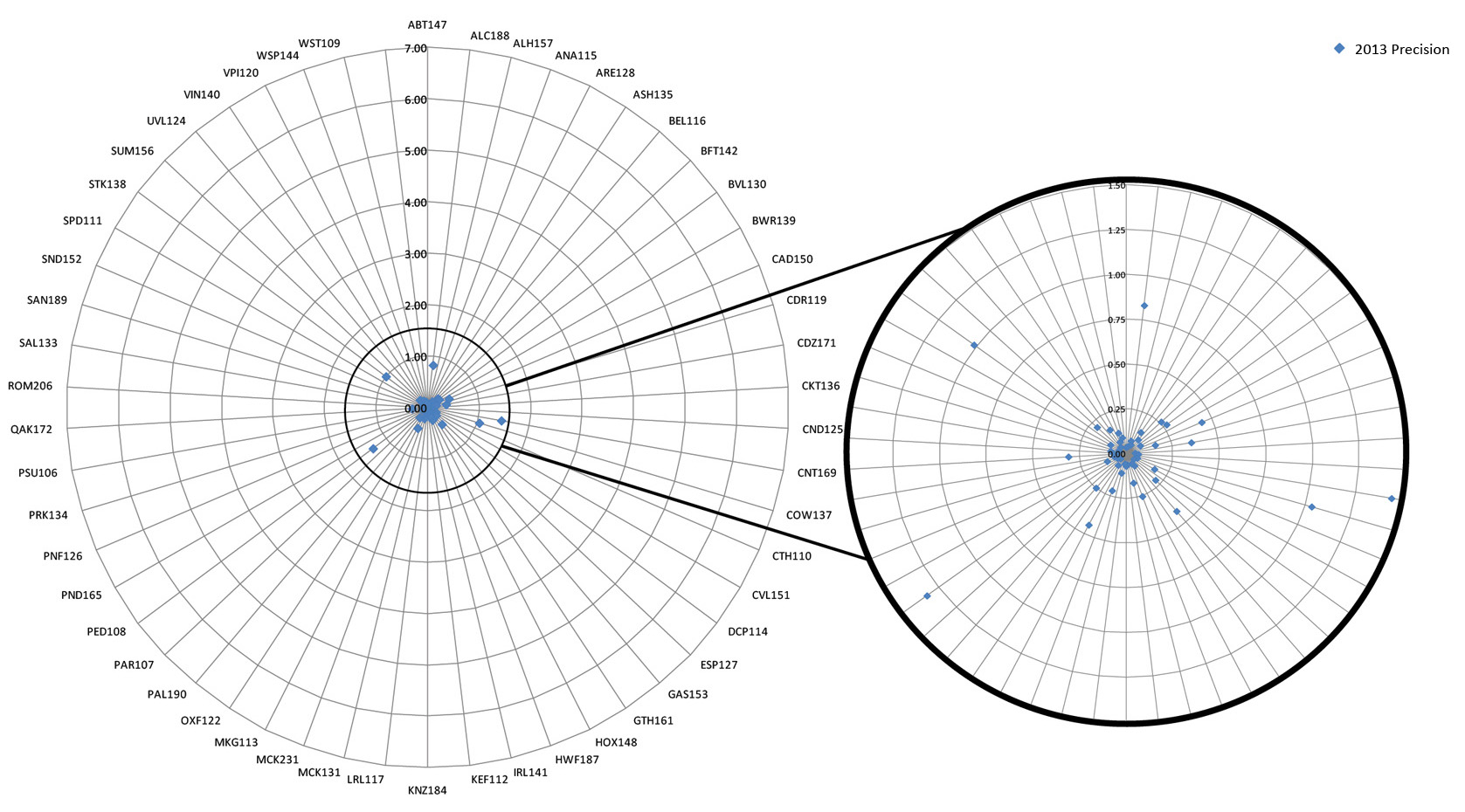
Ozone precision was estimated based on the acceptance criteria set forth in 40 CFR Part 58, Appendix A (EPA, 2010a). The O3 instrument was challenged with a known O3 concentration of 90 parts per billion (ppb) each day. The acceptance criterion is an upper 90 percent confidence limit (CL) for the coefficient of variation (CV) of 7 percent, i.e., 90 percent CL CV ≤ 7 percent. All EPA-sponsored sites met the precision acceptance criteria in 2013 (Figure 2-a).
Figure 2-a 2013 Precision (90 percent Confidence Limit of the Coefficient of Variation)
 Download Image
Note: QA program results for NPS-sponsored sites measuring O3 may be accessed at http://www.nature.nps.gov/air/monitoring/network.cfm
Eight-Hour Ozone Concentrations
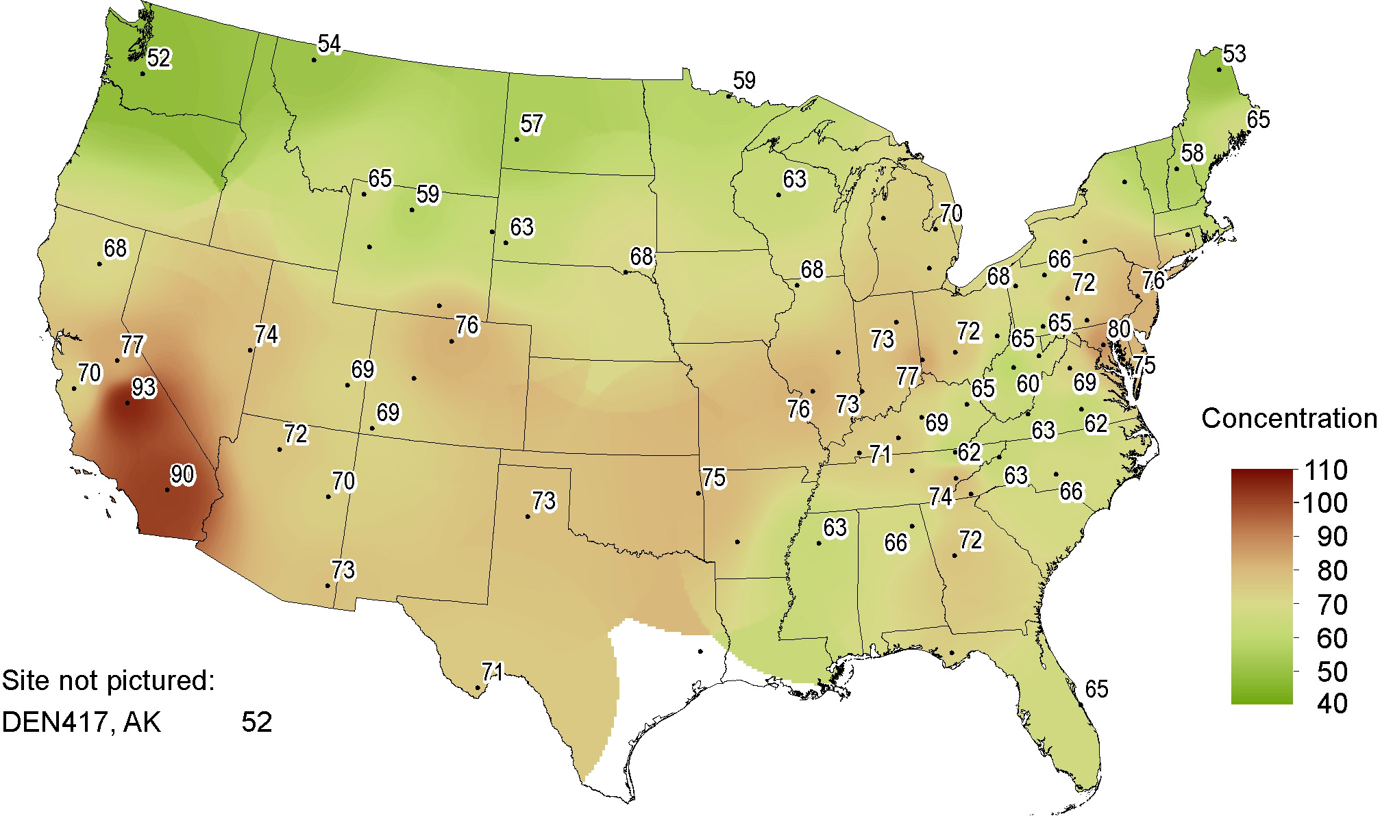
All CASTNET O3 data for 2011 through 2013 were measured using regulatory-compliant procedures and, therefore, are used to calculate design values and to gauge compliance with the NAAQS. O3 concentrations were not included on the maps in this chapter if the 3-year average was not available because of incomplete data; these sites are shown as dots with no value. Figure 2-1 presents 3-year averages of the fourth highest DM8A O3 concentrations for 2011 through 2013. Table 2-1 provides examples of sites with design values that exceed 75 ppb. Eight CASTNET sites measured exceedances of the O3 NAAQS.
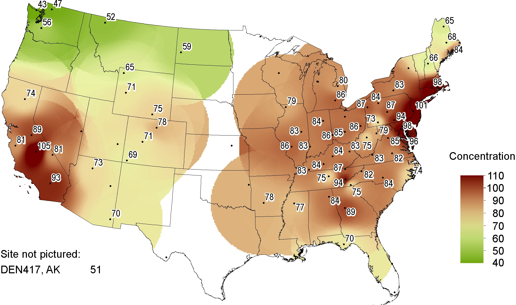
Three-year averages of the fourth highest DM8A O3 concentrations for 2000 through 2002 are presented in Figure 2-2 for comparison with the 2011 through 2013 values shown in Figure 2-1.
Figure 2-1 Three-year Average of Fourth Highest DM8A O3 Concentrations (ppb) for 2011–2013
 Download Figure
Figure 2-2 Three-year Average of Fourth Highest DM8A O3 Concentrations (ppb) for 2000–2002
 Download Figure
The period 2000 through 2002 was selected because it shows O3 concentrations prior to reductions in NOx emissions under the NOx SIP Call/NBP, which began in 2003 for the eastern United States.
All valid 2013 O3 concentrations that meet regulatory requirements are shown in Figure 2-3. Exceptional event determinations have not been finalized, and, therefore, any adjustments to these data as a result of exceptional events have been omitted. Again, exceptional events are unusual or naturally occurring situations that can affect air quality but are not reasonably controllable using standard techniques (EPA, 2013).
Table 2-1 Sites with 3-year Averages for 2011–2013 Greater than 75 ppb
| Site ID | State | Sponsor | 3-yr Average (ppb) |
|---|---|---|---|
| SEK430 | CA | NPS | 93 |
| JOT403 | CA | NPS | 90 |
| BEL116 | MD | EPA | 80 |
| YOS404 | CA | NPS | 77 |
| OXF122 | OH | EPA | 77 |
| ROM406 | CO | NPS | 76 |
| ALH157 | IL | EPA | 76 |
| WSP144 | NJ | EPA | 76 |
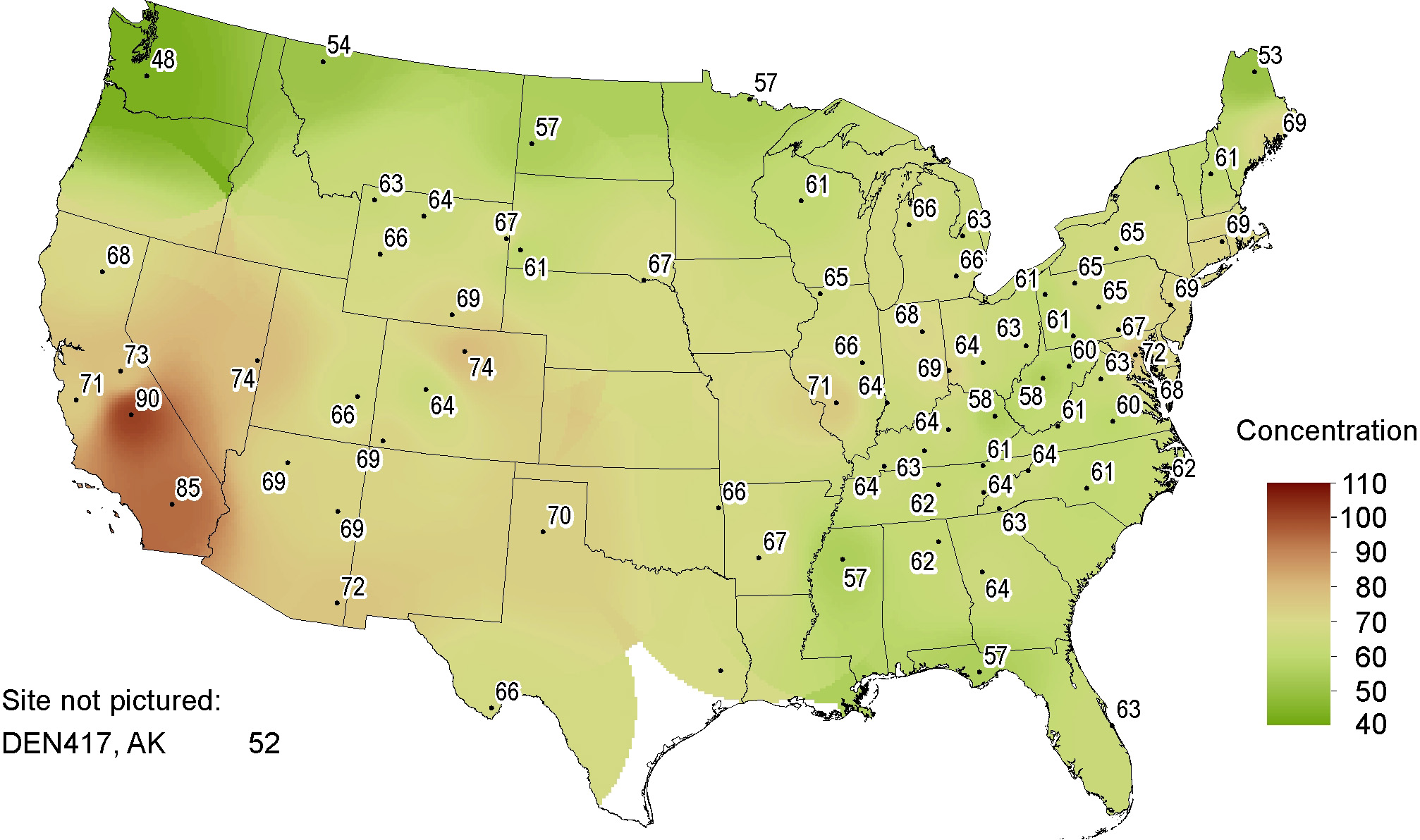
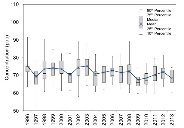
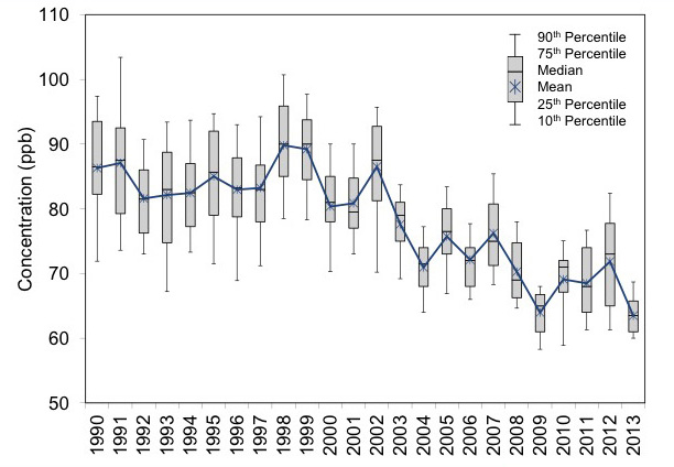
Figure 2-4 provides box plots depicting trends in 1-year mean values and distributions of fourth highest DM8A O3 concentrations from the 34 CASTNET eastern reference sites (right side) and 17 western reference sites (left side). The eastern O3 data show an overall reduction since 2002. The 2013 aggregate data point, 63 ppb, was the lowest level in the history of the network.
The western O3 data show an increase in O3 from the 2009 minimum through 2012, followed by a decrease in 2013. The 2013 average of the fourth highest DM8A O3 concentrations for the western reference sites was 68 ppb.
Figure 2-4 Trends in Fourth Highest DM8A O3 Concentrations
Cedar Creek State Park, WV (CDR119)
W126 Values for 2011 through 2013
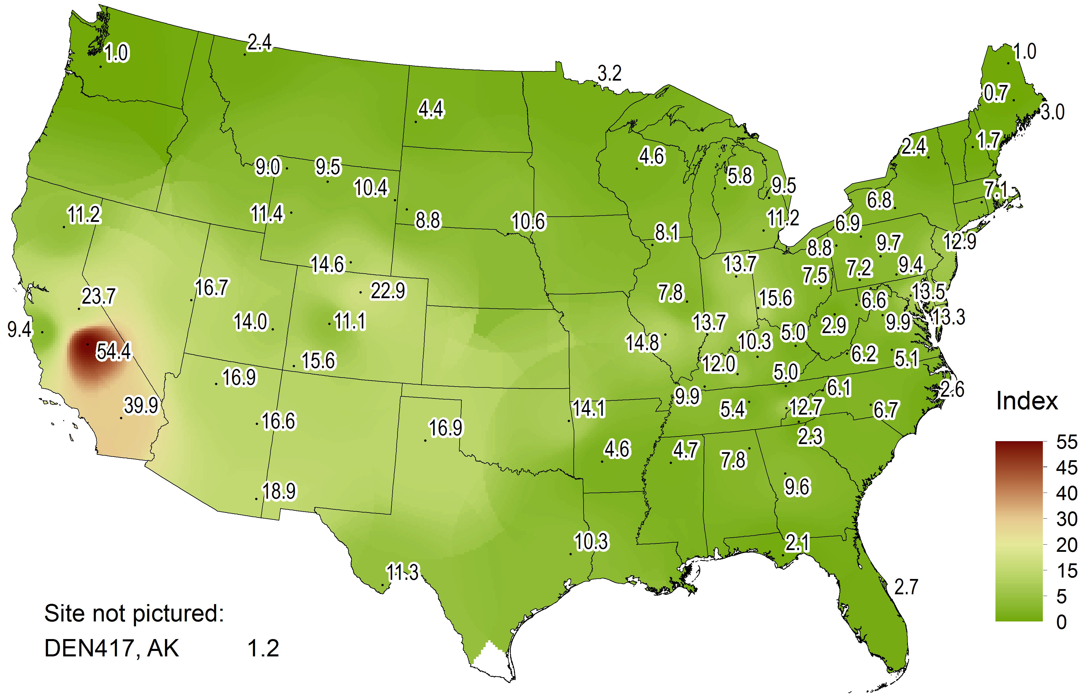
The W126 O3 exposure index is a cumulative, peak-weighted exposure indicator (Lefohn and Runeckles, 1987; EPA, 1996; 2006) for relating reduced vegetation yields to O3 exposure. W126 was developed as a seasonal metric from the sum of weighted hourly O3 values measured during the approximately 12-hour daylight period during the O3 season with the higher hourly concentrations being weighted more heavily than lower concentrations (EPA, 2010b). In this report, the W126 index is used to characterize exposure to O3 concentrations over a 3-month period during the O3 season for 2011 through 2013 and for 2013. The highest rolling 3-month W126 values for each site are presented for the two periods in Figures 2-b and 2-c.
W126 exposures (ppm-hour) were calculated using O3 values measured during the 12 hours from 8:00 a.m. to 8:00 p.m. in the months of May through September. First, the daily value for each site was calculated. The daily values were then used to calculate the monthly values for the months of May through September. The highest of the rolling 3-month sums for a consecutive 3-month period was the W126 value for each site. For reference, a W126 index value of 21 ppm-hour is associated with an approximate level of crop protection of no more than 10 percent yield loss in 50 percent of crop cases studied in the National Crop Loss Assessment Network (NCLAN) experiments (2013). A W126 index value of 13 ppm-hour is associated with an approximate level of crop protection of no more than 10 percent yield loss in 75 percent of NCLAN cases, keeping in mind that vegetative sensitivity to O3 varies between and within species. The proposed secondary NAAQS for O3 is identical to the primary standard of 65 to 70 ppb in order to provide protection for a W126 level of 13 to 17 ppm-hour, averaged over three years.
Sequoia National Park, CA (SEK430) north view
W126 values for the 3-year period 2011 through 2013 are shown in Figure 2-b. CASTNET sites in California and the western United States measured the higher W126 values. A value of 54.4 ppm-hour was recorded at SEK430, CA. Seven sites in the East measured values greater than 13 ppm-hour.
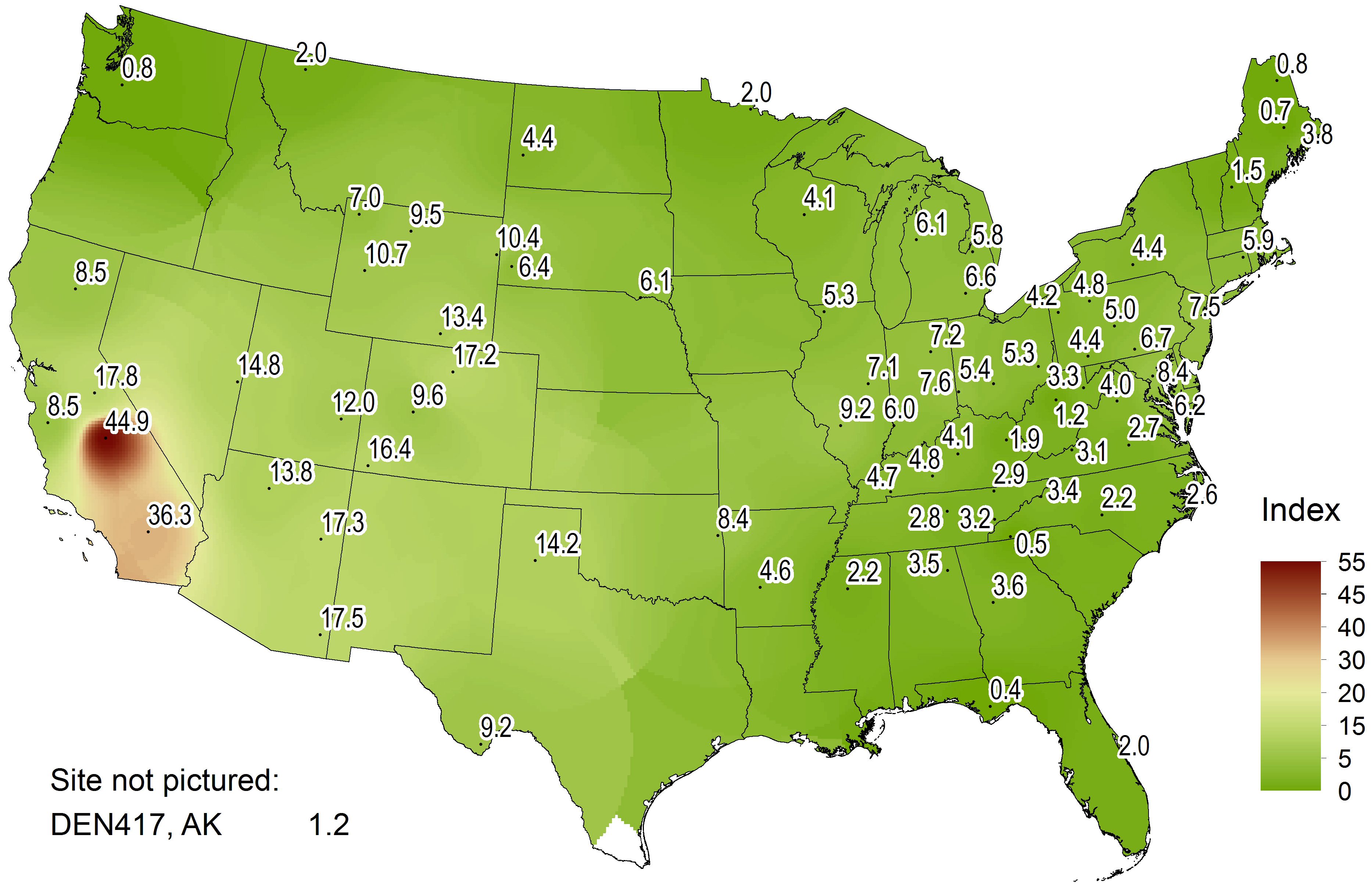
W126 levels for 2013 for CASTNET sites are presented in Figure 2-c. The higher W126 values were measured in California and at western sites in high terrain. The highest W126 value (44.9 ppm-hour) was measured at SEK430. W126 values for 2013 were lower than the 2011–2013 values. O3 concentrations measured at high-elevation sites typically persist during the night because dry deposition and scavenging of O3 by nitric oxide are low at night (AMEC, 2003; Talbot et al., 2005). Nighttime dry deposition is low because shallow boundary layers typically do not form at elevated sites, and scavenging is low because little fresh nitric oxide is available to react with the existing O3. The persistence of moderate O3 concentrations at night produces steady exposure and high W126 levels.
Chapter 3: Trace-level Gas Concentrations
Continuous trace-level gas air quality monitors were operated at a total of eight CASTNET sites during 2013. EPA sponsored routine trace-level gas monitoring at six CASTNET sites. NPS operated one trace-level gas monitoring system in Kentucky. Additionally, as part of the Beaufort total nitrogen study, nitrogen oxide/total reactive oxides of nitrogen, nitrogen oxides, and nitrogen dioxide were measured at the EPA-sponsored site at Beaufort, NC through May 2013. The measurements at these sites were performed to (1) support EPA NCore monitoring, (2) provide data to understand atmospheric processes such as ozone and fine particulate matter formation, and (3) generate regional model input. Air quality monitors were operated continuously to measure trace-level concentrations. Total reactive oxides of nitrogen was measured at all eight sites, sulfur dioxide at three sites, and carbon monoxide at two sites. Total reactive oxides of nitrogen concentrations were highest at two suburban sites and lowest at the high-elevation, mountainous sites.
During 2013, Teledyne Advanced Pollution Instrumentation analyzers were deployed at the six EPA-sponsored CASTNET sites with trace-level gas monitoring. Table 3-1 lists the site locations, start dates, and the trace-level gas parameters measured at each site. Hourly O3 concentrations were measured at all sites. These data were sampled continuously and archived as 1-hour values. Trace-level monitoring was performed by NPS at Mammoth Cave National Park, KY (MAC426) during 2013. Operation of trace-level instrumentation as part of a short-term study at Beaufort, NC (BFT142) is documented in the “Measurements of Atmospheric NH3 and NOy/NOx/NO2 and Deposition of Total Nitrogen at the Beaufort, NC CASTNET Site (BFT142)” report (Baumgardner et al., 2014), also called the Beaufort Nitrogen Study. The deployment and sampling schedule for the BFT142 site can be found in the report. In addition, NO/NOy measurements were taken by other federal and state agencies at CASTNET or nearby sites in Tennessee, North Dakota, South Dakota, and Maine.
Table 3-1 Trace-level Gas Monitoring Sites Operated during 2013
| Site Location | Start Dates | Measurements |
|---|---|---|
| Beltsville, MD (BEL116) | March 2005 | NO/NOy and SO2 |
| Mammoth Cave NP, KY* (MAC426) | May 2009 | NO/NOy, SO2, and CO |
| Beaufort, NC** (BFT142) | February 20012 | NO/NOy/NOx/NO2 |
| Bondville, IL (BVL130) | July 2012 | NO/NOy, SO2, and CO |
| Huntington Wildlife Forest, NY (HWF187) | November 2012 | NO/NOy |
| Pinedale, WY (PND165) | May 2013 | NO/NOy |
| Cranberry, NC (PNF126) | October 2013 | NO/NOy |
| Rocky Mountain National Park, CO (ROM206) | October 2013 | NO/NOy |
Note:
* Operated by NPS during 2013
** Operated during the Beaufort Nitrogen Study through May 2013
NOy, a precursor for O3 and PM2.5, is defined as NOx [NO + nitrogen dioxide (NO2)] plus NOz (HNO3, nitrous acid, peroxyacetyl nitrate, peroxyproyl nitrate, other organic nitrates, and nitrite). NOy is converted to NO using a thermal converter and then measured by chemiluminescence. Continuous SO2 is measured using ultraviolet fluorescence, and CO is measured by gas filter correlation. Data are used to assess the effectiveness of emission reductions, to understand PM2.5 formation processes, for model evaluation, and as a comparison with the CASTNET filter pack measurements.
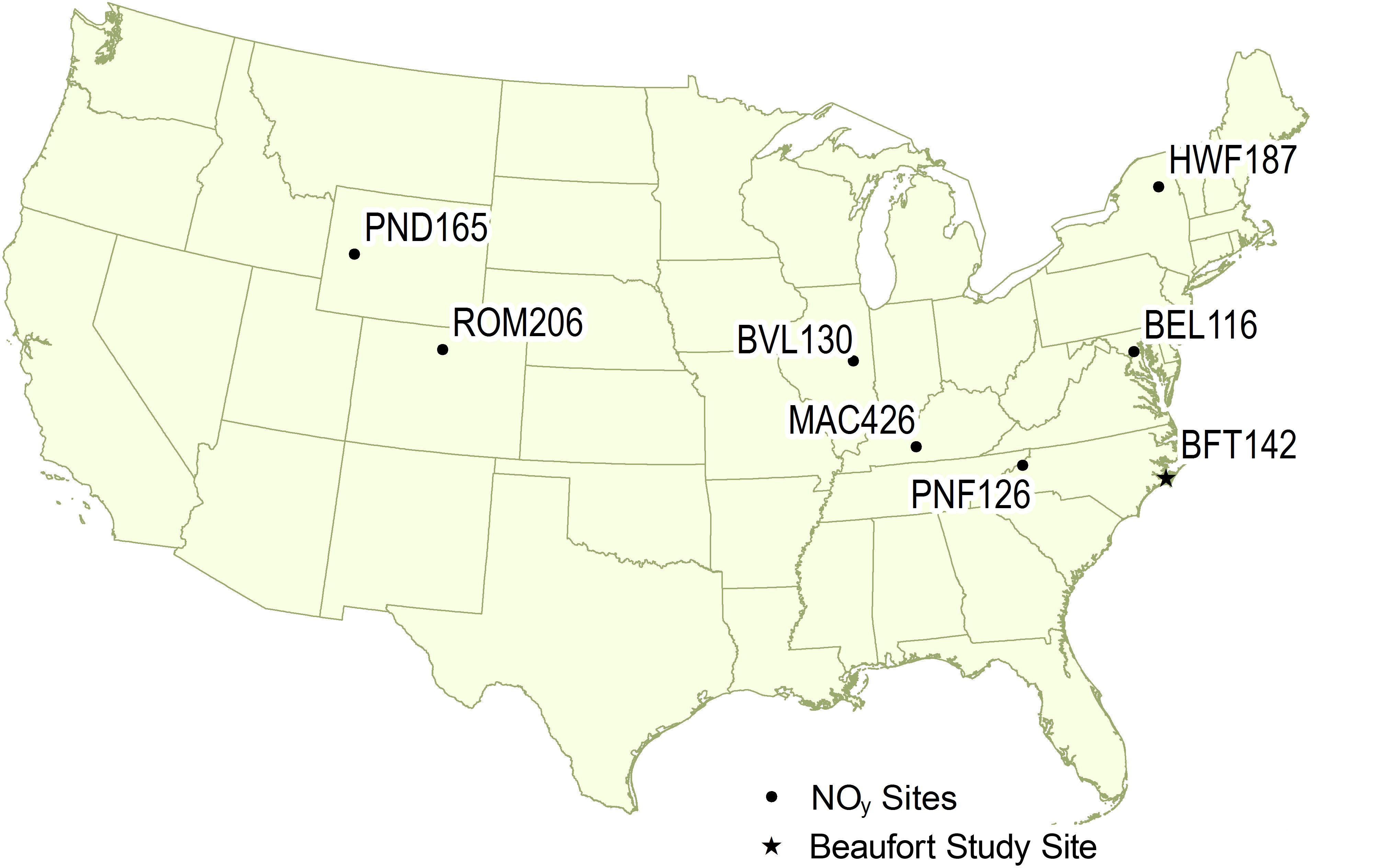
Figure 3-1 provides a map of the CASTNET trace-level gas monitoring site locations. All sites were operated according to the CASTNET QAPP Appendix 11, Procuring, Installing, and Operating NCore Air Monitoring Equipment at CASTNET Sites (AMEC, 2012; 2013c). The CASTNET QAPP and all related appendices and the Beaufort Nitrogen Study Report (Baumgardner et al., 2014).
Quality Assurance Program Results
Trace-level Gas Concentrations
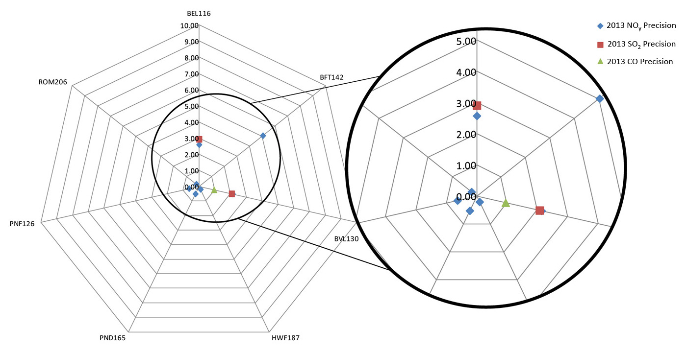
Trace-level gas precision was estimated based on the acceptance criteria set forth in 40 CFR Part 58 Appendix A (EPA, 2010a) for NOy (including the criteria pollutant NO2), SO2, and CO. The NOy instrument was challenged with a known concentration of 15 ppb NO each day, the SO2 instrument with 25 ppb of SO2, and the CO instrument with 250 ppb of CO. The acceptance criterion is an upper 90 percent confidence limit (CL) for the coefficient of variation (CV) of 10 percent, i.e., 90 percent CL CV ≤ 10 percent. Precision data for only EPA-sponsored sites are plotted in Figure 3-a. These sites met the acceptance criteria in 2013.
Figure 3-a 2013 Trace-level Gas Precision (90 Percent Confidence Limit of the Coefficient of Variation)
 Download Figure
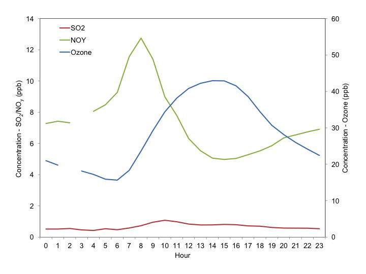
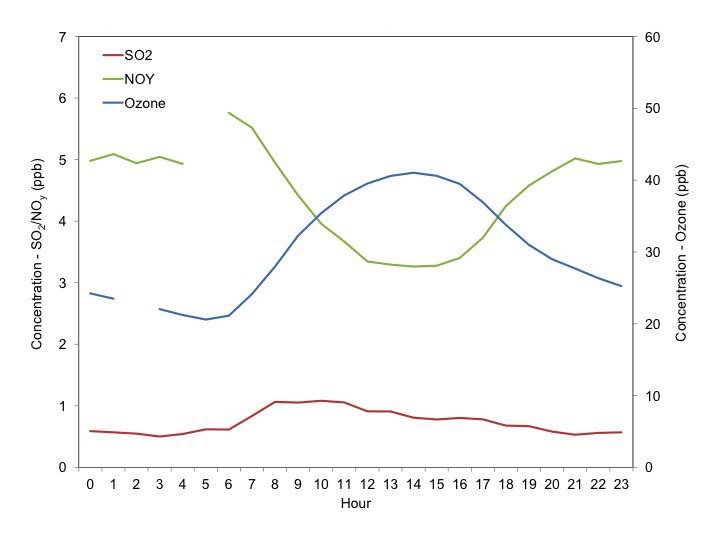
Four of the sites operated trace-level gas monitors for the entire year. These sites are BEL116, BVL130, MAC426, and HWF187. Figures 3-2 and 3-3 present 2013 annual average hourly composite diurnal profiles of SO2, NOy, and O3 for BEL116 and BVL130, respectively. Figures 3-4 and 3-5 show the 2013 annual average hourly composite diurnal profiles of NOy and O3 for MAC426 and HWF187, respectively. Figures 3-6 through 3-8 show composite diurnal profiles of NOy and O3 for PNF126 (November through December 2013), PND165 (May through December 2013), and ROM206 (November through December 2013), respectively. The profiles in Figures 3-2 through 3-8 were constructed by averaging all values from the same hour for their respective time periods. The figures illustrate how the differences in geography and terrain/elevation affect the evolution of photochemically reactive pollutants in the boundary layer.
Huntington Wildlife Forest, NY (HWF187)
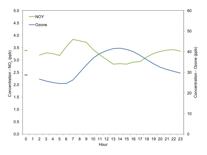
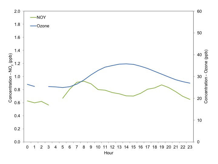
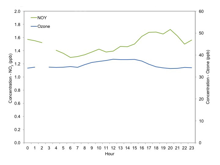
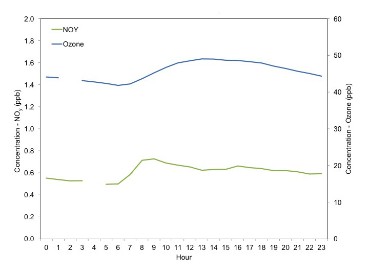
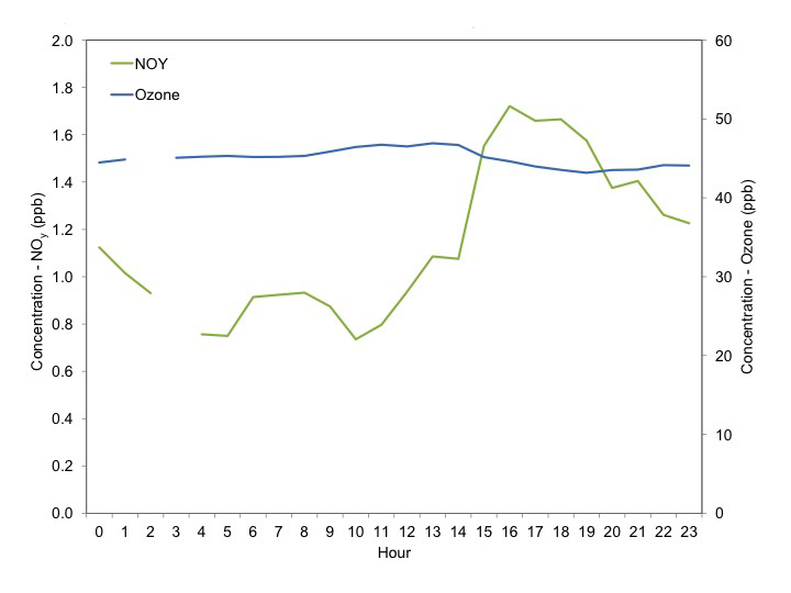
Table 3-2 Summary of 2013 Minimum and Maximum Values from Diurnal Charts
| Site Location* | Site Elevation (meters) | NOy(ppb) | O3(ppb) | ||
|---|---|---|---|---|---|
| Min | Max | Min | Max | ||
| BEL116, MD | 47 | 5.0 | 12.7 | 16 | 43 |
| BVL130, IL | 213 | 3.3 | 5.8 | 21 | 41 |
| MAC426, KY | 243 | 2.8 | 3.8 | 25 | 42 |
| HWF187, NY | 497 | 0.6 | 0.9 | 25 | 36 |
| PNF126, NC | 1,216 | 1.3 | 1.7 | 34 | 38 |
| PND165, WY | 2,386 | 0.5 | 0.7 | 42 | 49 |
| ROM206, CO | 2,742 | 0.7 | 1.7 | 43 | 47 |
Note: * Sites are listed in order of Elevation
Trace-level NOy and Ozone
The minimum and maximum mean composite NOy and O3 concentrations shown in Figures 3-2 through 3-8 are summarized in Table 3-2. The sites are listed in order of elevation. The highest NOy concentrations were measured at BEL116, an eastern suburban site in a region with relatively high NOx emissions from mobile sources. Low NOy values were recorded at the four rural sites in New York, North Carolina, Wyoming, and Colorado. The seven profiles in Figures 3-2 through 3-8 illustrate the loss of O3 during the late afternoon and nighttime hours and its production during daylight. The diurnal change was less pronounced at the four rural sites. The BEL116 site observed the largest nighttime loss and subsequent highest daytime production, an average increase of about 27 ppb of O3 for 2013. The BVL130 data illustrate a typical diurnal relationship between NOy and O3 concentrations with peak NOy concentrations associated with NOx emissions (e.g., vehicle traffic) in the morning and evening and peak O3 concentrations in the afternoon. The data from MAC426 also show a diurnal evolution with the highest NOy concentrations in the morning and at night. These data look similar to measurements made at an urban site.
Data were collected at PND165, ROM206, and PNF126 during a few months in 2013, i.e., eight months at PND165 and two months at both ROM206 and PNF126. More recent data are discussed in the 2014 CASTNET Quarterly Data Reports (AMEC, 2014a; 2014c). The highest O3 concentration was measured at PND165. The concentrations measured at the three sites with the highest elevations show less 24-hour variation than the other four sites because of the absence of nighttime O3 loss/depletion mechanisms near the high-elevation monitors (Talbot et al., 2005). Nighttime dry deposition is low because shallow boundary layers typically do not form at these high-elevation sites, and scavenging is low because fresh nitric oxide is not available to react with O3. The ROM206 data suggest a large production or transport of NOy around sunset. There are no significant NOx sources in the area. The increase in NOy is likely a result of the transformation of polluted air masses from the Front Range Urban Corridor and the associated late afternoon upslope flow.
Trace-level and Filter Pack Sulfur Dioxide Concentrations
Hourly average trace-level concentrations of SO2 were collected at the BEL116 and BVL130 sites during 2013. The comparison of trace-level continuous data with filter pack concentration data is performed routinely to evaluate both measurements. Trace-level continuous and filter pack SO2 values were compared for each site. Figure 3-9 provides a bar chart that compares weekly aggregated SO2 data from the continuous analyzer with weekly integrated filter pack SO2 measurements at the BEL116 site. There was a positive relationship between the continuous analyzer and filter pack measurements with a regression line:
y = 0.8125x + 0.0246.
The correlation coefficient for the two sets of measurements is 0.6136.
Beltsville, MD (BEL116)
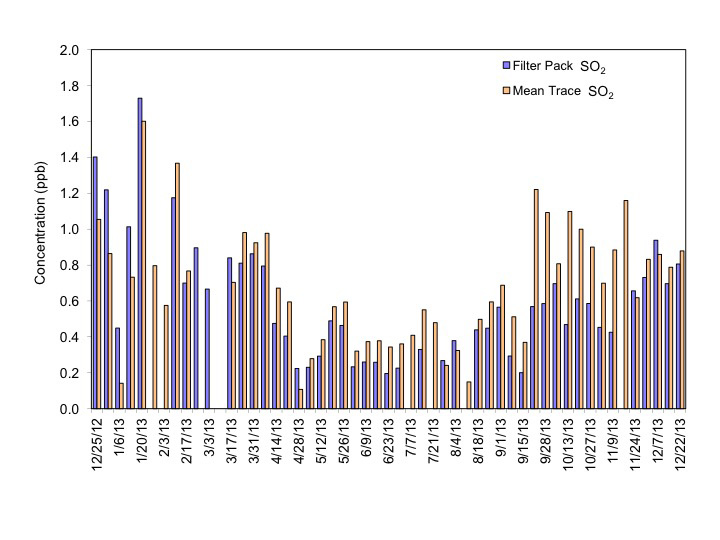
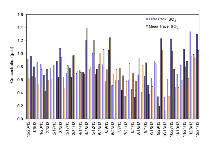
Figure 3-10 provides a bar chart for the BVL130 site that compares weekly mean SO2 data from the continuous analyzer with weekly filter pack SO2 measurements. The figure shows higher filter pack concentrations in early 2013 through mid-March and again from early September through December. The continuous and filter pack SO2 data for 2013 have a regression line:
y = 0.6616x + 0.2815.
The correlation coefficient for the two sets of measurements is 0.4370.
Enhancements to Air Quality and Deposition Monitoring in New York
The State of New York has long been committed to monitoring air pollution and atmospheric deposition across the state. Such data are used to gauge compliance with the NAAQS, contribute to air quality forecasts, and assess the impacts of emission reductions of SO2 and NOx precursors to O3, PM2.5, regional haze, and acidic deposition. Two recent initiatives will allow New York to continue this work in an efficient manner over the coming years, as well as be more responsive to changing monitoring needs and priorities.
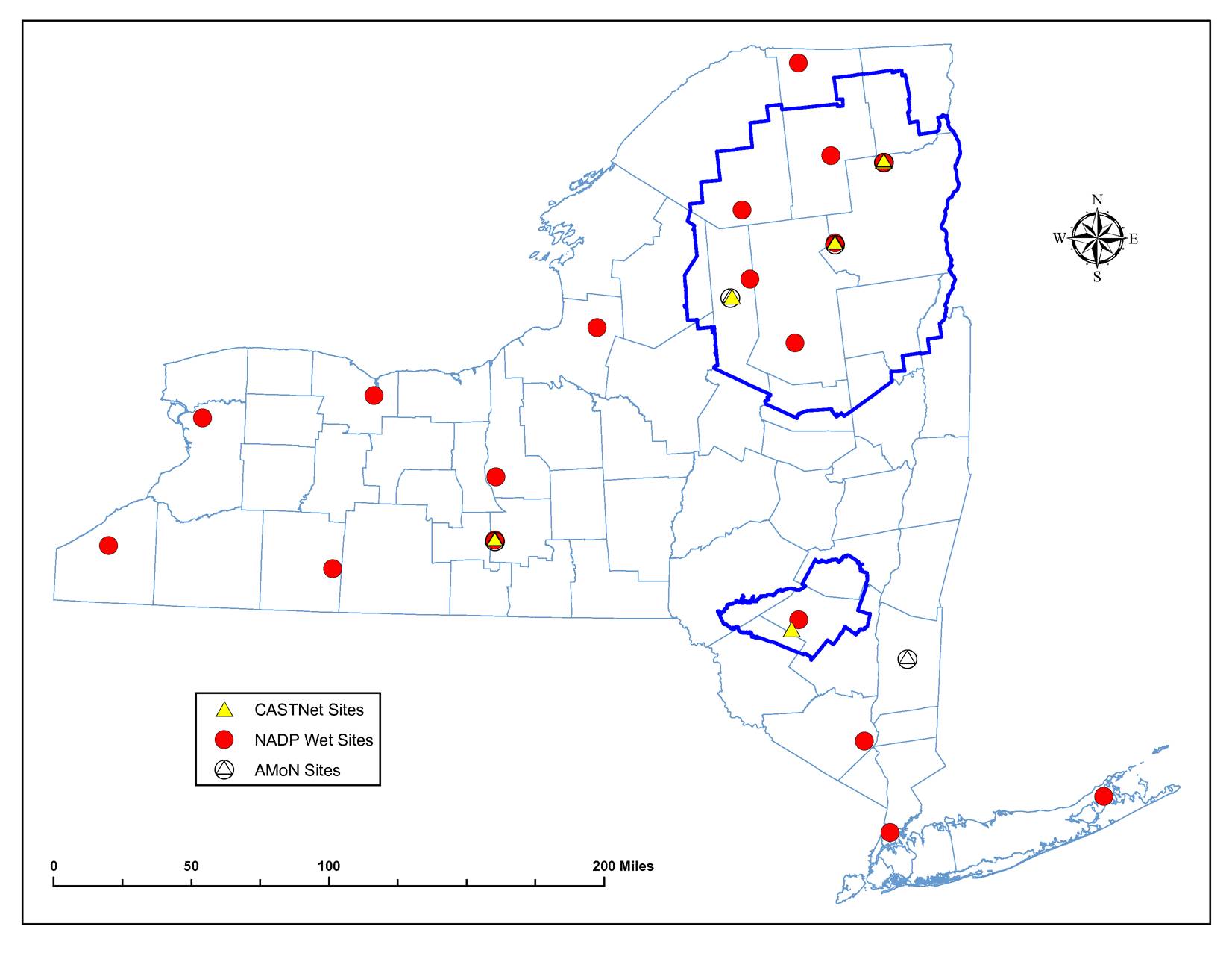
The first development relates to wet deposition monitoring. After more than 25 years of maintaining an independent wet deposition network, in late 2012, the New York State Department of Environmental Conservation (NYSDEC) began to convert some sites to the NADP protocols (Figure 3-b). Three NTN samplers have been added to urban and suburban locations – Amherst (suburb of Buffalo), Rochester, and New York City. Three other NTN sites were established in the Adirondack Mountain region of northern New York – Paul Smith’s College, Piseco Lake, and the State University of New York (SUNY)-Environmental Science and Forestry (ESF) Ranger School in Wanakena. This transition to the NADP protocols ensures consistent deposition monitoring at all sites across New York, with a particular focus on sensitive ecosystems. Except for the site at Wanakena, these wet deposition sites also collect data on criteria air pollutants, air toxics, various hydrocarbons, and/or Hg ambient concentrations and wet Hg deposition.
Second, NYSDEC decided to collect data to calculate an aquatic acidification index (AAI) based on an EPA proposed pilot field program designed to better understand this index. EPA’s plans also called for a passive AMoN sampler and a continuous NOy monitor at the existing HWF187 CASTNET site in the central Adirondack Mountains. In an effort to characterize the variability and impacts of wet and dry deposition in this region, NYSDEC has added CASTNET and AMoN passive NH3 samplers to two additional sites in the Adirondack region. The first is at Nicks Lake Campground (NIC001), which is approximately 15 kilometers from the NTN site at Moss Lake, located in the southwestern Adirondacks, a region particularly impacted by acid deposition. The other site is collocated with the NTN sampler at Whiteface Mountain (WFM105), a site representative of the highest elevations in the northeastern Adirondacks. The NTN site at Wanakena and the CASTNET and AMoN monitors at Nicks Lake are shown in Figure 3-c.
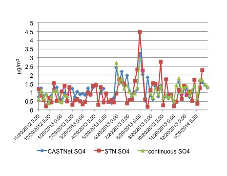
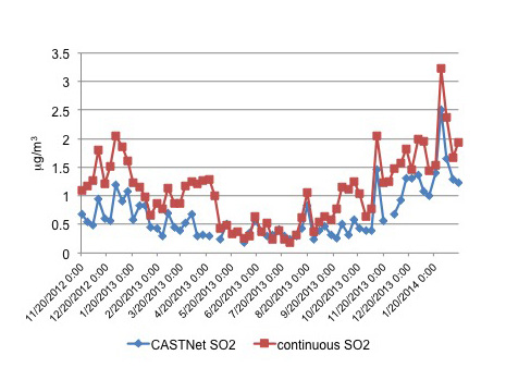
A number of co-pollutants are also monitored by the State of New York at the WFM105 site, including hourly SO2 and SO42- from pulsed fluorescence analyzers and 24-hour PM2.5 speciation (1 day in 6) from a Speciation Trends Network (STN) sampler. A comparison of these two parameters, averaged over the corresponding CASTNET sampling week, covering the period November 2012 to February 2014, is shown in Figure 3-d. While there is generally good agreement for integrated SO42- over this time period, differences in SO2 are more pronounced. These differences, likely associated with aerosol composition and temperature and humidity changes, are still being investigated. The results also show that the continuous SO2 measurements were higher than the CASNET filter pack concentrations.
Figure 3-b Locations of NTN, CASTNET, and AMoN sites in New York and outlines (blue) of the Adirondacks and Catskill Park
 Download Figure
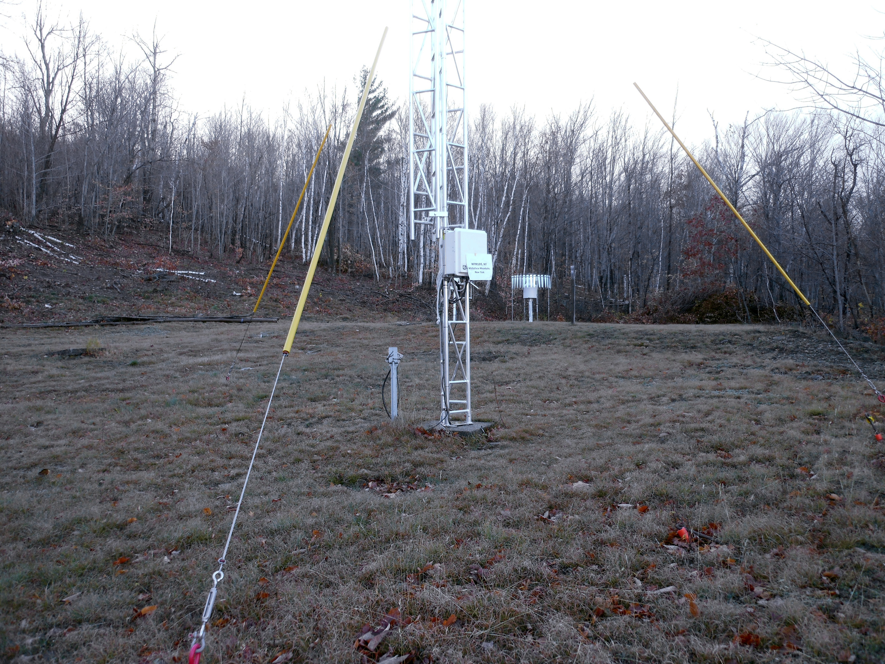
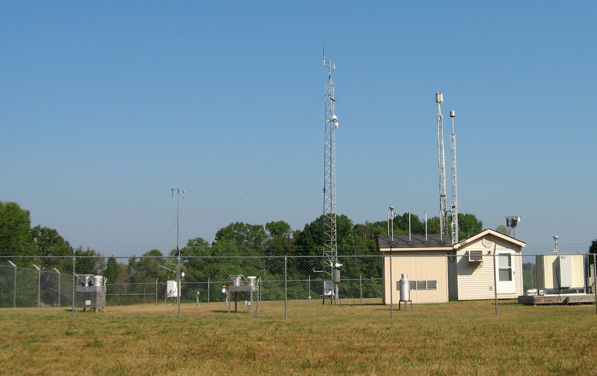
Whiteface Mountain, NY (WFM105)
Figure 3-c NTN sampler at the SUNY-ESF Ranger School in Wanakena (left) and CASTNET/AMoN samplers at the Nicks Lake Campground (right) in the Adirondack Mountain Region
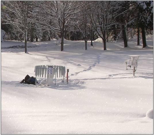
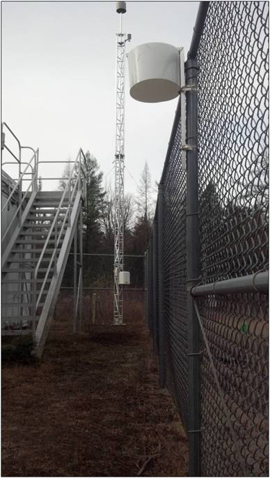
Figure 3-d Comparison of CASTNET, STN, and Continuous SO42- (left) and CASTNET and Continuous SO2 (right) at WFM105, November 2012 to February 2014
Trace-level NOy and Filter Pack Total Nitrate Concentrations
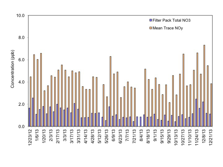
HNO3 and particulate NO3- are measured on CASTNET filter packs, and the sum is reported as total NO3-. Because HNO3 and particulate NO3- are measured as components of NOy, NOy concentrations should always be higher than total NO3- levels; the ratio of NOy to total NO3- should always be greater than 1.0. A comparison of weekly mean continuous NOy concentrations with filter pack total NO3- levels at BVL130 was used to evaluate the measurements (Figure 3-11). The NOy concentrations were consistently higher than the total NO3- levels, as expected. The results are similar for the other six sites. The weekly total NO3- concentrations, the average weekly NOy levels, and their ratios are listed in Table 3-3. These were calculated as the average of all valid weekly filter pack concentrations and the average of mean NOy values matching the run time of the weekly filter packs. Weekly NOy levels were higher than the weekly total NO3- concentrations with ratios of NOy to total NO3- varying from 4.06 at BVL130 to 9.70 at BEL116. The highest concentration (1.18 ppb) of total NO3- at BVL130 resulted in the lowest ratio of 4.06.
Table 3-3 Summary of Total NO3- and NOy Measurements for 2013
| Site Location | Total NO3 (ppb) | NOy (ppb) | Ratio |
|---|---|---|---|
| BEL116, MD | 0.78 | 7.41 | 9.70 |
| BLV130, IL | 1.18 | 4.44 | 4.06 |
| MAC426, KY | 0.74 | 3.21 | 4.34 |
| HWF187 | 0.18 | 0.70 | 4.28 |
| PNF126, NC | 0.31 | 1.49 | 5.28 |
| PND165, WY | 0.17 | 0.61 | 4.21 |
| ROM206, CO | 0.11 | 1.24 | 9.45 |
Mammoth Cave National Park, KY (MAC426)
Figure 3-11 Comparison of BVL130 Weekly Mean NOy and Total NO3- Concentrations for 2013
 Download Figure
Bondville, IL (BVL130)
Update on the Ammonia Monitoring Network (AMoN)
Gaseous NH3 has become increasingly important in the past decade because reactive NH3 concentrations and depositions have shown little change in the face of tightening standards for NOx emissions (Puchalski et al., 2011). NH3 is the most prevalent base gas in the atmosphere and is released into the air from a variety of biological sources, as well as from industrial and combustion processes, with the largest sources of emissions in the agricultural sector. Although NH3 has beneficial applications, such as in NH3-based fertilizer use, it can also have a detrimental effect on the environment when it reacts with acidic ions such as SO42- and NO3- to form ammonium sulfate [(NH4)2SO4] and ammonium nitrate (NH4NO3) particles, which are significant components of PM2.5. NH3 and NH4+ particles also contribute to visibility degradation and the atmospheric deposition of nitrogen to sensitive ecosystems. Human health effects include short-term eye and lung irritation and long-term cardiovascular system impacts through inhalation of the PM2.5.
Despite the importance of NH3 in atmospheric chemistry, the impact of NH3 on ecosystems, and possible human health effects, routine monitoring of ambient NH3 was not performed until recently. In response to a 2007 US-Canada workshop on NH3, NADP initiated AMoN as a special study in the fall of 2007 with fourteen sites. AMoN was officially approved as a NADP network in October 2010, and currently (as of December 2014) the network consists of 66 sites across the United States. To determine the proper sampling device for AMoN, NADP evaluated the performance of three passive samplers: Adapted Low-cost Passive High Absorption (ALPHA), Radiello, and Ogawa. Results from the ALPHA and Radiello samplers were compared with results from annular denuders, and results from the Ogawa samplers were compared with results from a continuous-trace level NH3 analyzer. The three passive samplers were also compared with each other. While the passive samplers yielded reasonably precise and accurate ambient NH3 data, the NADP decided to deploy Radiello samplers due to the ease of sample preparation and extraction, making these samplers less labor intensive and, therefore, more cost-effective. The samplers are deployed for 2 week periods and do not require electricity or a data logger for operation.
The objectives of AMoN are to:
- Assess long-term trends in ambient NH3 concentrations and depositions of reduced nitrogen species,
- Evaluate atmospheric models,
- Provide better estimates of total nitrogen inputs to ecosystems,
- Assess changes in atmospheric chemistry due to SO2 and NOx emission reductions,
- Assess compliance with PM2.5 standards, and
- Evaluate possible long-term climate effects due to spatial and temporal trends of NH3 gas in the atmosphere.
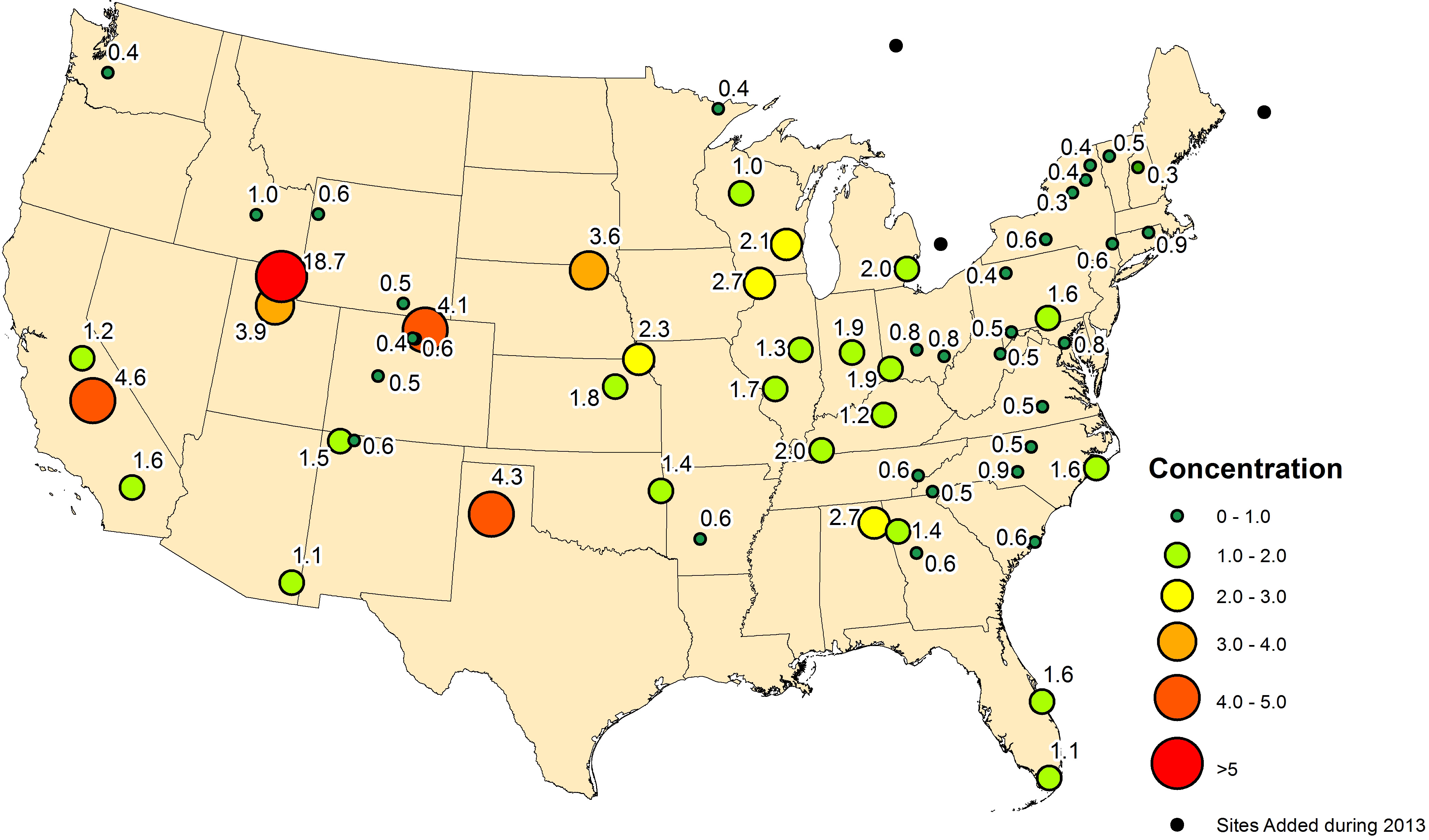
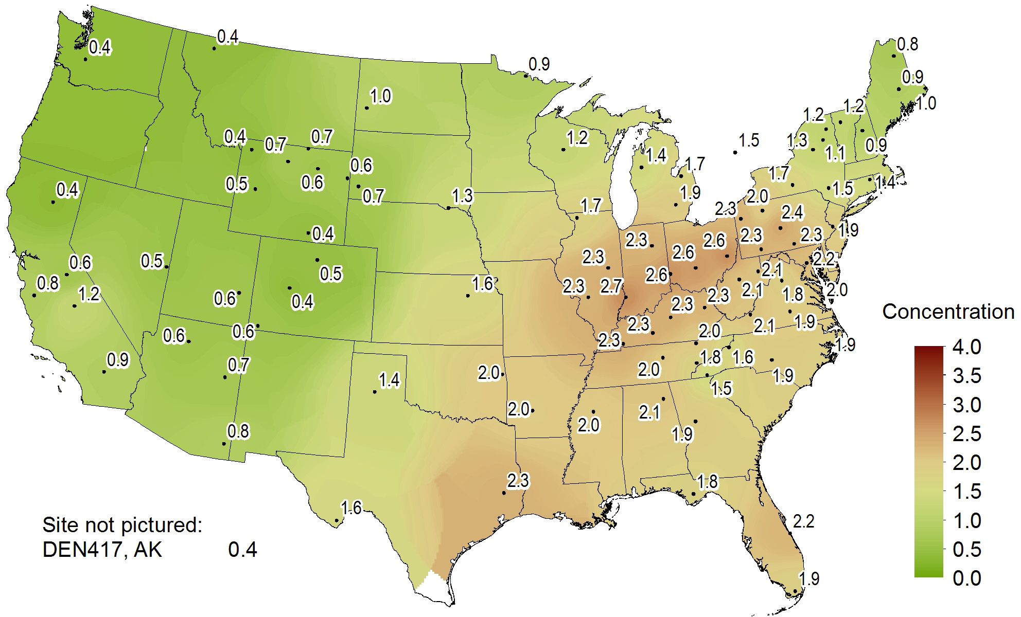
Average annual NH3 concentrations for 2013 for the 60 sites that met completeness requirements are plotted in Figure 3-e and show a wide range of concentrations ranging from a low of 0.3 micrograms per cubic meter (µg/m 3 ) of air in New Hampshire and New York to a high of 18.7 µg/m 3 in northern Utah. The Utah site measured an exceptionally high annual average. The next highest values ranged from 3.6 to 4.6 µg/m 3 at five western sites. The highest concentration east of the Mississippi occurred at the northern Alabama site and the northern Illinois site (2.7 µg/m 3 ). No regional patterns were observed, other than the western sites had a combined average annual 2013 concentration of 2.7 µg/m 3, and the eastern sites had an annual average of 1.1 µg/m 3. Even if the value for northern Utah was excluded, the western sites had a higher annual average (1.8 µg/m 3 ) for 2013. Patterns of high local NH3 concentrations are largely influenced by agricultural operations (e.g., cattle feeding and crop production).
Ten AMoN sites have been operating since late 2007. However, because of data incompleteness, annual averages for these sites could not be calculated until beginning with 2009 data. Table 3-a presents 2009 and 2013 annual averages and the percent differences in concentrations from 2009 to 2013. All 10 sites measured higher concentrations in 2013 than 2009 and support the observation that reactive NH3 concentrations have shown little change despite lower SO2 and NOx emissions, which in turn have resulted in lower atmospheric (NH4)2SO4 and NH4NO3 and perhaps higher NH3 concentrations. These results also support the continued need for an NH3 network since concentrations are likely increasing, at least in certain locations (Puchalski et al., 2011).
Table 3-a Average Annual NH3 Concentrations at 10 AMoN Sites (2009 and 2013)
| Site ID* | 2009 | 2013> |
|
||
|---|---|---|---|---|---|
| Concentration
(ug/m 3) |
N | Concentration
(ug/m 3) |
N | Percent
Changed |
|
| CO13 | 3.4 | 27 | 4.1 | 26 | +20 |
| IL11 | 1.1 | 26 | 1.3 | 26 | +17 |
| IN99 | 1.2 | 27 | 1.9 | 23 | +53 |
| MN18 | 0.3 | 27 | 0.4 | 27 | +59 |
| OH02 | 0.6 | 27 | 0.8 | 24 | +36 |
| OH27 | 1.4 | 27 | 1.9 | 26 | +34 |
| OK99 | 1.2 | 27 | 1.4 | 26 | +15 |
| SC05 | 0.3 | 27 | 0.6 | 24 | +135 |
| TX43 | 2.9 | 27 | 4.3 | 26 | +48 |
| WI07 | 1.8 | 27 | 2.2 | 26 | +18 |
Note:
*AMoN site information can be found at http://nadp.sws.uiuc.edu/amon/. By convention, the first two alphabetic characters of the NADP site identification are the state abbreviation where the site is located.
N = number of samples
Because the largest source of NH3 emissions is the agricultural sector (including feedlot operations and fertilizer application), reactive NH3 concentrations and depositions do not exhibit the downward trend shown by sulfur and other nitrogen species (AMEC, 2013a), which are more closely tied to power and industrial sector emissions and track relatively well with the emission reductions mandated by CAAA requirements. Atmospheric NH3 concentrations and depositions are more complex because NH3 deposition is bidirectional; NH3 can be emitted and re-emitted from vegetation and soils and deposited from the atmosphere. In order to keep improving our understanding of the role of NH3 in air quality and the resultant impacts, both ecological and human health related, NADP’s future plans for AMoN include growing the network to 300+ sites to cover all sensitive ecoregions of the United States. Also, a greater number of sites will generate additional data to improve the ability to evaluate air quality and deposition models.
Stilwell, OK (OK99/CHE185)
Chapter 4: Atmospheric Concentrations
Weekly average concentrations of sulfur dioxide, particulate sulfate, nitric acid, particulate nitrate, particulate ammonium, particulate chloride, and four base cations were measured using 3-stage filter packs at 92 CASTNET monitoring stations during 2013. Trends in mean annual sulfur dioxide, sulfate, total nitrate (nitric acid plus nitrate), and ammonium aggregated over 34 eastern and 17 western reference sites are shown using box plots. The sulfur and nitrogen pollutants measured at the 34 eastern reference sites declined over the 24-year period from 1990 through 2013. Measured annual mean concentrations of sulfur dioxide and sulfate have decreased steadily with major annual reductions since 2005. Concentrations of total nitrate began to drop in 2000 in response to nitrogen oxides emission reduction mandates and have continued to decline slowly. Sulfur dioxide, sulfate, total nitrate, and ammonium concentrations measured at the 17 western reference sites declined over the last 18 years, 1996 through 2013. The reduction in sulfur pollutants is consistent with the reduction in sulfur dioxide emissions. The reduction in nitrogen pollutants did not correspond to the reduction in oxides of nitrogen emissions as closely as sulfur dioxide concentrations tracked sulfur dioxide emissions because, in addition to power plants, transportation and other combustion sources produce oxides of nitrogen emissions and contribute to ambient nitrogen pollutants.
Maps of 2013 annual mean concentrations of SO2, SO42-, total NO3- (HNO3 + NO3-), and NH4+ are presented in this chapter. Additional maps of 2013 quarterly mean concentrations are provided in CASTNET quarterly data reports (AMEC, 2013b; 2013d; 2014b; 2014d). Trends in annual mean concentrations over the 24-year period (1990 through 2013) were derived from measurements from the 34 CASTNET eastern reference sites and for the period 1996 through 2013 from data measured at 17 CASTNET western reference sites. See Appendix A for the designated reference sites.
Sulfur Dioxide Concentrations
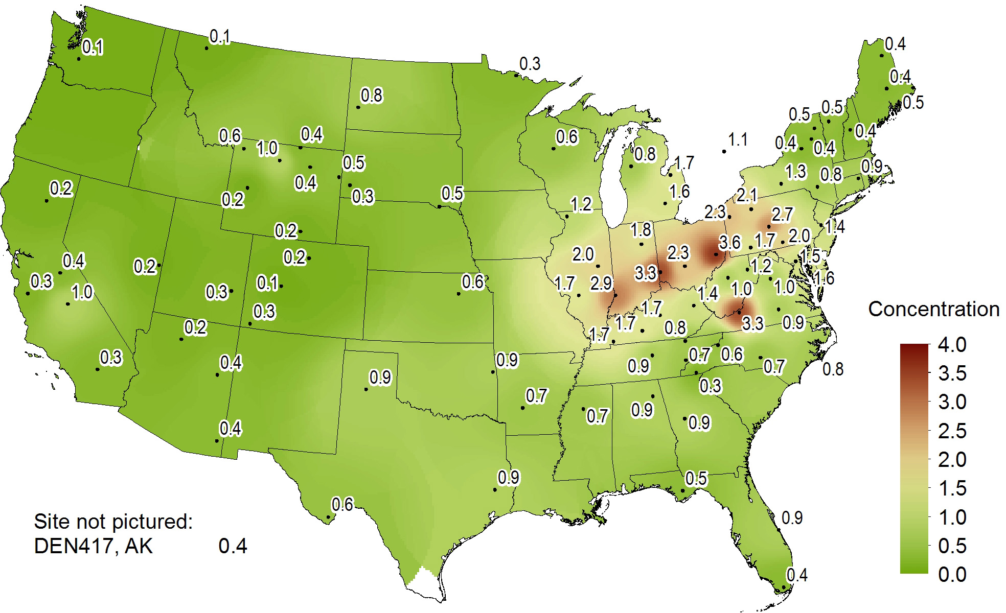
2013 annual mean SO2 concentrations are shown in Figure 4-1. Annual mean concentrations were highest in the Midwest near the Ohio River.
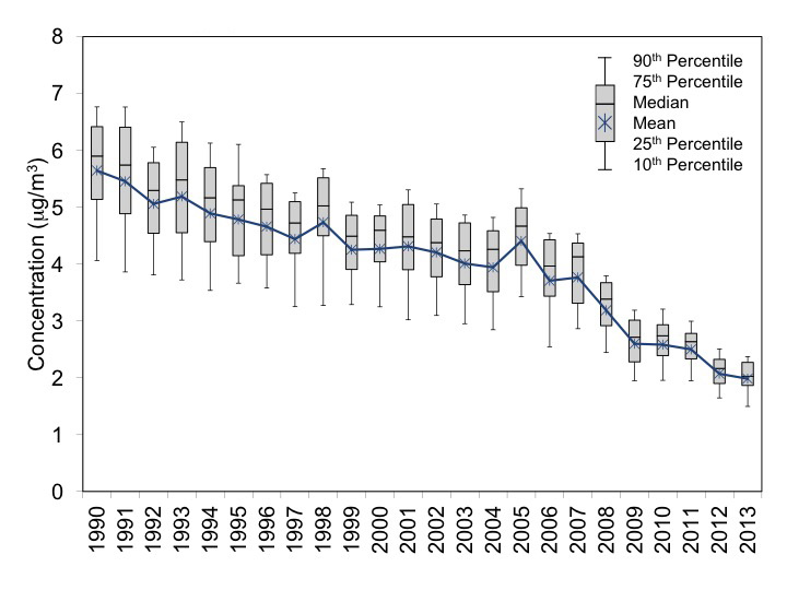
Box plots of annual mean SO2 concentrations aggregated over the 34 eastern reference sites from 1990 through 2013 (right side) and the 17 western reference sites from 1996 through 2013 (left side) are depicted in Figure 4-2. The y-axes on the western and eastern plots have different scales because concentrations measured at the western CASTNET sites were much lower than those measured at the eastern sites. Each box presents the mean and median concentrations and the 10th, 25th, 75th, and 90th percentiles for that year.
Three-year mean concentrations for the eastern reference sites for 1990–1992 and 2011–2013 were 8.9 µg/m 3 and 1.7 µg/m 3, respectively. This change constitutes an 80 percent reduction in 3-year mean SO2 concentrations between the two periods. The 2013 mean level of 1.4 µg/m 3 was the lowest mean value measured by the eastern reference sites in the history of the network and represents a significant decline over the last eight years from the 2005 concentration of 6.1 µg/m 3.
Unionville, MI (ULV124)
Quality Assurance Program Results
Precision of Filter Pack Measurements
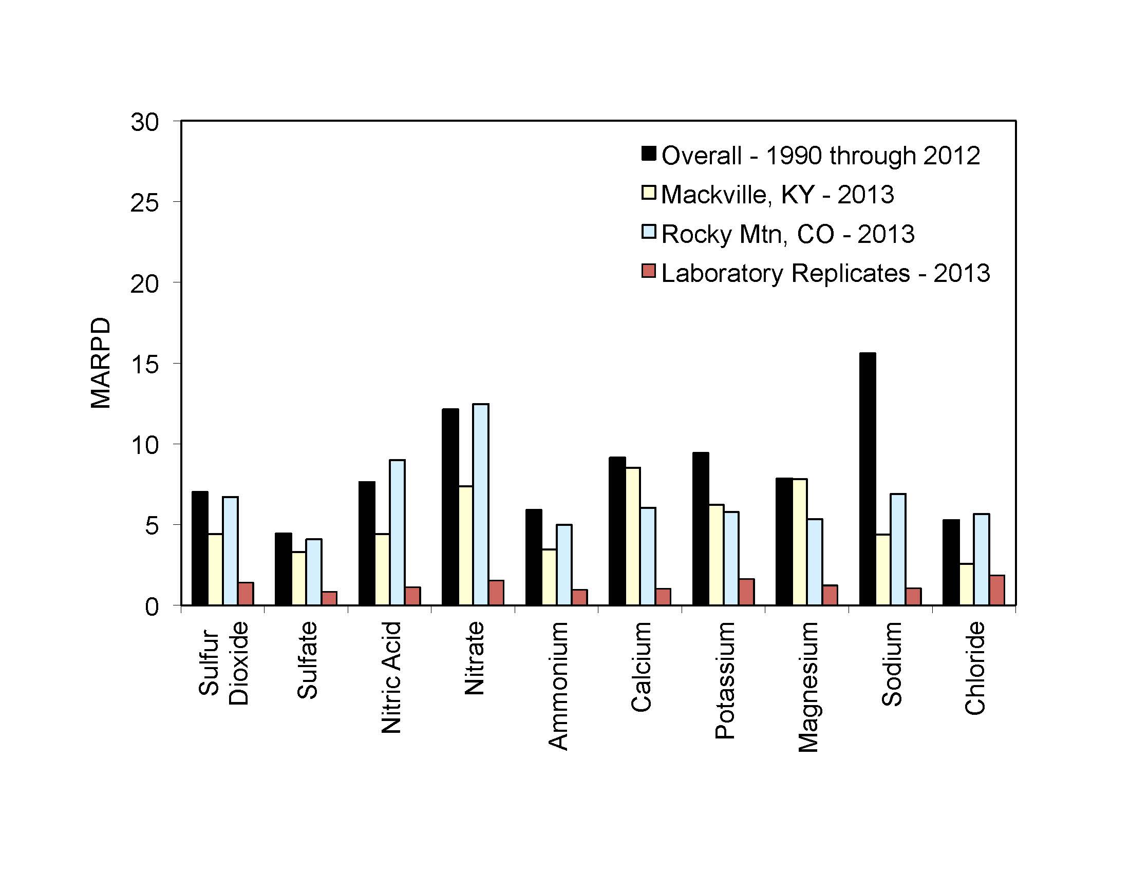
Historical (1990 through 2012) mean absolute relative percent difference (MARPD) data for all 11 collocated site pairs operated over the history of the network and the 2013 data for the current collocated sites at MCK131/231 and ROM406/206 are provided in the bar chart in Figure 4-a. The precision criterion is a MARPD of 20 percent. Historical and 2013 measurements met the criterion for each analyte.
The 2013 analytical precision results for 10 measurements are also presented in Figure 4-a. The results were based on analysis of 5 percent of the samples that were randomly selected for replication in each batch. The results of in-run replicate analyses were compared to the original concentration results. The laboratory precision data met the 20 percent measurement criterion.
Figure 4-a Historical and 2013 Precision Results for Atmospheric Concentrations and Laboratory Replicate Samples
 Download Figure
Data Completeness
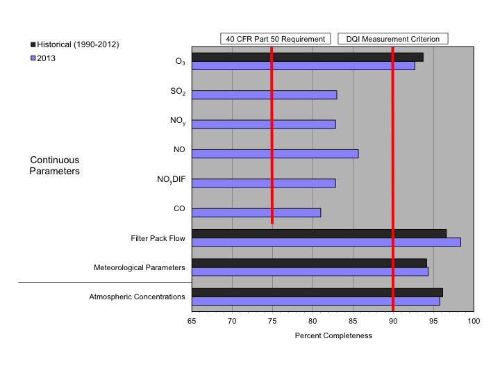
Completeness is defined as the percentage of valid data points obtained from a measurement system relative to total possible data points. The CASTNET measurement criterion for completeness requires a minimum completeness of 90 percent for every measurement for each quarter. The historical results and the results for 2013 are given in Figure 4 b. Historical results are not available for trace-level gas measurements. The completeness criterion was met for atmospheric (filter pack) and O3 concentrations, filter pack flow, and meteorological measurements. Completeness of trace-level gas measurements (Chapter 3) met the completeness requirements of 40 CFR Part 50 (EPA, 2008b).
Figure 4-b Historical and 2013 Percent Completeness of Measurements
(black bars are 1990–2012)
 Download Figure
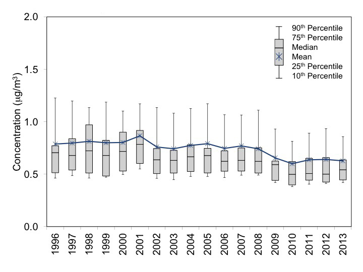
The box plots for the western reference sites indicate a decline in annual mean SO2 concentrations aggregated over the 17 sites. Three-year mean SO2 concentrations for 1996–1998 and 2011–2013 were 0.6 µg/m 3 and 0.3 µg/m 3, respectively. This change constitutes a 54 percent reduction in 3-year mean SO2 concentrations at the CASTNET western reference sites over the 18 years.
The 2013 average sulfur dioxide concentration for the eastern reference sites was 1.4 µg/m 3, the lowest level in the history of the network. The eastern sulfur dioxide data show a substantive decline since 1997. The reduction (80 percent) in sulfur dioxide concentrations is consistent with the reduction (84 percent) in sulfur dioxide emissions from EGUs operating in Illinois, Indiana, Kentucky, Ohio, West Virginia, and Pennsylvania, suggesting an approximately linear relationship between concentrations and emissions.
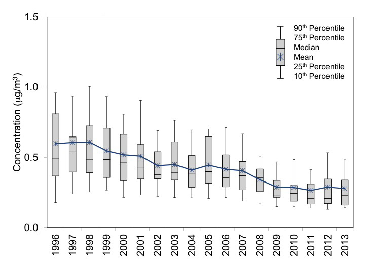
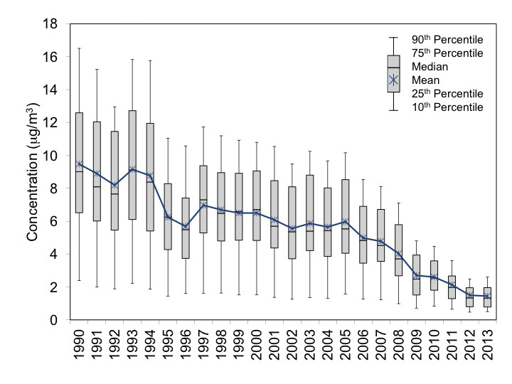
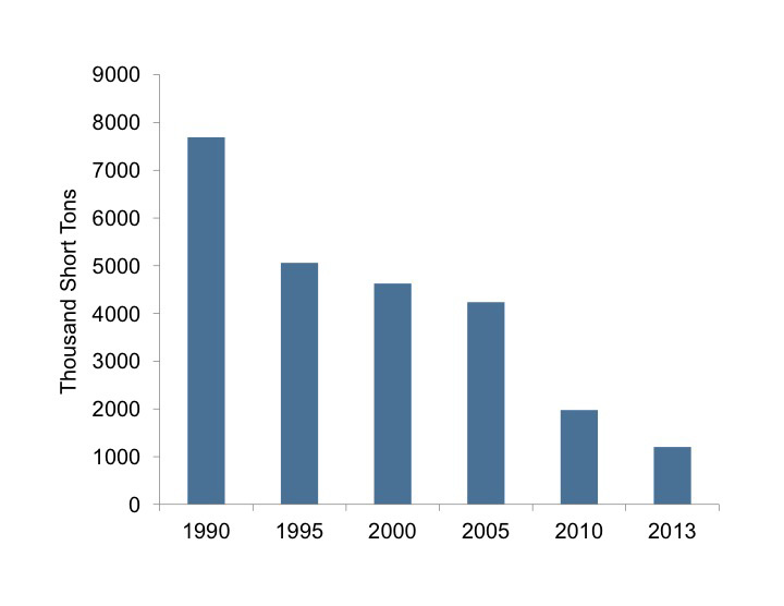
Figure 4-3 Trend in Annual Composite SO2 Emissions from Regulated EGUs Operating in Illinois, Indiana, Kentucky, Ohio, West Virginia, and Pennsylvania
 Download Figure
Note: Data from 477 EGUs in 1990, 415 in 1995, 519 in 2000, 751 in 2005, 747 in 2010, and 687 in 2013 were used to construct the bar chart.
Figure 4-3 illustrates the trend in SO2 emissions from regulated EGUs from 1990 through 2013 aggregated over six states (Illinois, Indiana, Kentucky, Ohio, West Virginia, and Pennsylvania). The 24-year decline in aggregated emissions for the six states was 84 percent, which is consistent with the 80 percent reduction (Figure 4-2) in annual mean SO2 concentrations aggregated over the CASTNET eastern reference sites and suggests an approximately linear relationship between SO2 concentrations and emissions.
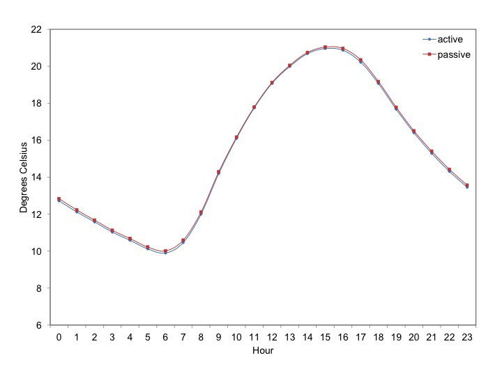
A Comparison of Temperature Measurements from Collocated Mechanically and Naturally Aspirated Sensors Operated at Three CASTNET Sites
EPA discontinued meteorological measurements, with the exception of 9-m temperature measurements, at all but four EPA-sponsored CASTNET sites over the period September 2010 through October 2012. Most of the meteorological monitoring had been discontinued by December 2010, although a few sites operated meteorological instruments until March 2013. The 9-m temperature measurements were continued at all sites to support filter pack measurements. NPS and BLM are continuing meteorological data collection at their sites.
The 9-m temperature measurements at EPA sites were switched from active, mechanically aspirated resistance-temperature device (RTD) sensors to passive, naturally aspirated RTD sensors. The switch was made to avoid operational and maintenance efforts and the associated costs. Of additional benefit, it eliminated the need for a separate tower for temperature measurements only. Unlike the actively aspirated sensors, the passively aspirated sensors can be located on the tilt-down sampling tower. The weight of the blower and blower housing for the active, mechanically aspirated sensors makes these sensors too heavy for installation on the tilt-down sampling towers. The 9-m temperature sensors are moved to the tilt-down sampling towers based on attrition and the CASTNET calibration schedule (see the CASTNET QAPP Table 2-11, AMEC, 2013c; 2012). Eventually, all temperature sensors will be the passive, naturally aspirated type with the exception of the sensors used at the four sites with complete meteorological measurements. Currently, about half of the EPA-sponsored sites have been converted to passive sensors.
Long-term cost savings are being realized because maintenance costs for the meteorological towers and blower motors have been eliminated. The passive shields used to replace the active shields were obtained from the discontinued relative humidity sensors. Reusing the shields avoided the need to incur new capital expenses.
Prior to beginning the switch to the passive, naturally aspirated sensors, collocated mechanically fan aspirated (active) and naturally aspirated (passive) temperature measurement systems were operated at three EPA sites for at least two years. The results are shown in Table 4-a.
Table 4-a A Comparison of Temperature Measurements from Collocated Mechanically Aspirated and Naturally Aspirated Sensors
| Site ID | Start Date | End Date | Active (°C) | Passive (°C) | Average
Difference (°C) |
Number of
Comparisons |
Percent
Complete |
|---|---|---|---|---|---|---|---|
| BEL116, MD | 07/30/11 | 08/14/13 | 13.73 | 13.84 | -0.11 | 16,575 | 93 |
| BVL130, IL | 09/06/11 | 09/08/13 | 11.91 | 11.88 | 0.03 | 17,264 | 98 |
| PAL190, TX | 11/01/11 | 11/109/13 | 15.27 | 15.36 | -0.10 | 17,821 | 99 |
Note: °C = Degrees Celsius
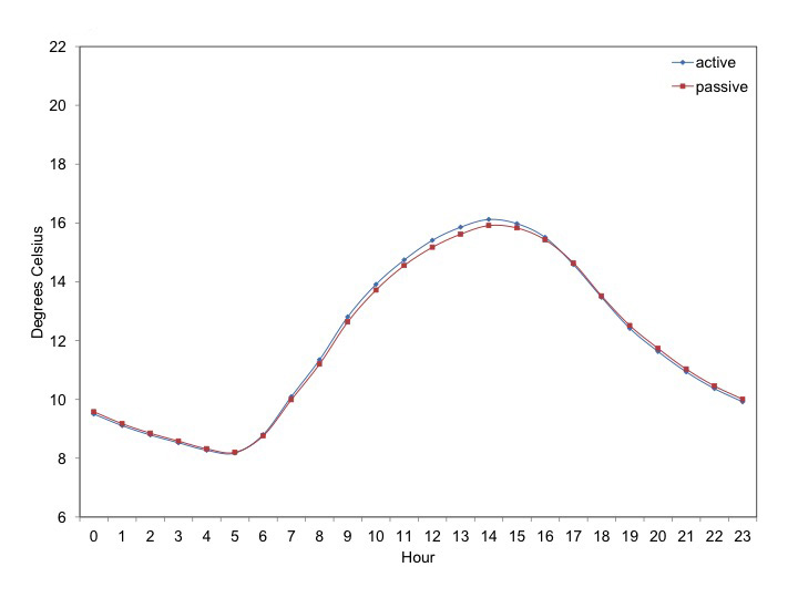
The average difference in temperature measurements between the active and passive samplers was less than 1.0 percent for all three sites. Figures 4-c through 4-e present composite diurnal plots of temperature values for the three active and three passive sensors operated at the three sites for their entire periods of performance. The profiles in these three figures were constructed by averaging all values from the same hour for the approximate 2-year period. The results show the temperature data from the active and passive samplers were comparable and demonstrate that use of the passive temperature devices to support the filter pack measurements is acceptable.
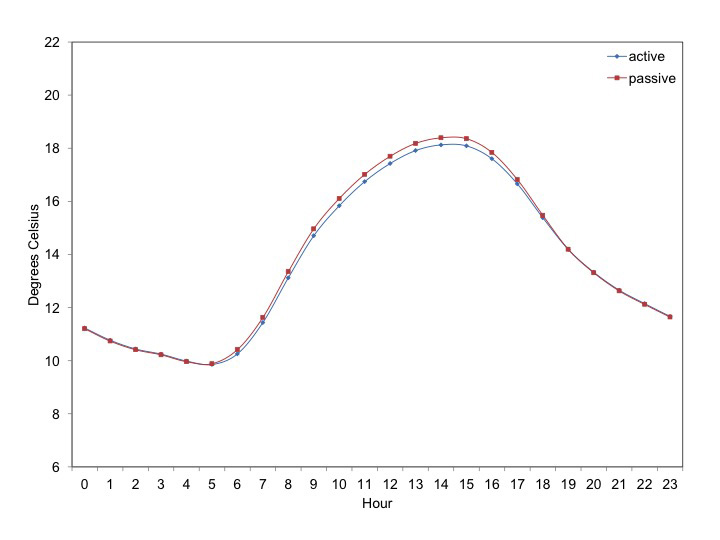
Figure 4-d Composite Diurnal Temperature Profiles September 2011 through September 2013
 Download Figure
Figure 4-e Composite Diurnal Temperature Profiles November 2011 through November 2013
 Download Figure
Particulate Sulfate Concentrations
Figure 4-4 shows a map of 2013 mean annual particulate SO42- concentrations. Figure 4-5 provides box plots of annual mean SO42- concentrations from the 34 eastern reference sites and 17 western reference sites. The right side shows the trend in measurements from the eastern reference sites. The figure shows a substantial decline in SO42- over the 24 years. Of particular note, concentrations declined rapidly from 2005 through 2012. The difference between 3-year means from 1990–1992 to 2011–2013 represents a 59 percent reduction in SO42- from 5.4 µg/m 3 to 2.2 µg/m 3, respectively. The 2013 mean SO42- level of 2.0 µg/m 3 was the lowest in the history of the network.
The box plots for the western reference sites are provided on the left side of Figure 4-5. The boxes show a 20 percent reduction in annual mean SO42- concentrations aggregated over the 17 sites with 1996–1998 and 2011–2013 concentrations of 0.8 µg/m 3 and 0.6 µg/m 3, respectively.
The 2013 average sulfate concentration for the eastern reference sites was 2.0 µg/m 3, the lowest level in the history of the network. The eastern sulfate data show a substantive decline since 1998. Sulfate concentrations declined more slowly than sulfur dioxide concentrations at the eastern reference sites. Western sulfate concentrations were lower and decreased at a slower rate than concentrations measured at the eastern sites.
Figure 4-5 Trends in Annual Mean SO42- Concentrations
Scenic view from Perkinstown, WI (PRK134)
Air Quality Studies in National Parks in the Bakken Formation
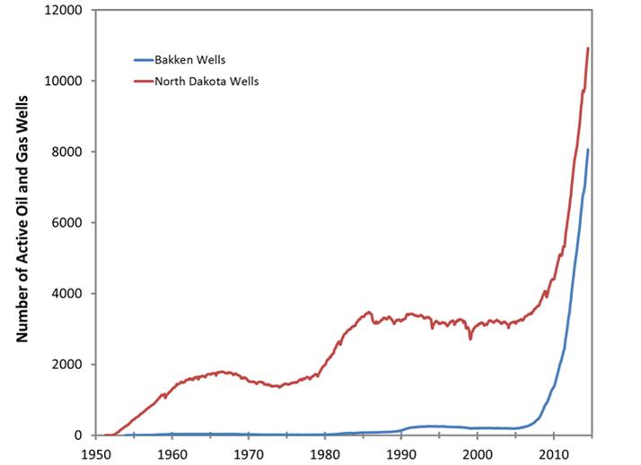
The Bakken formation contains billions of barrels of oil and gas trapped in rock and shale in North Dakota, Montana, Saskatchewan, and Manitoba. New horizontal drilling and hydraulic fracturing methods have allowed access to these oil and gas deposits. This has led to an exponential growth in the number of wells and production of oil, with most of the activity occurring in North Dakota. As of October 2014, there were more than 10,000 active wells in North Dakota (Figure 4-f), primarily located in the Bakken region. Significant drilling is also occurring in Montana.
Although oil is the primary commodity coming from the Bakken, there is also a large amount of associated natural gas. Unlike many areas with energy development, in North Dakota there is not yet an established infrastructure to transport this natural gas. Until recently, approximately 30 percent of the gas was burned off in flares (Figure 4-g), generating significant gaseous and particle emissions. In 2014, the North Dakota Industrial Commission required Gas Capture Plans to be included with all Applications for a Permit to Drill permit renewals (North Dakota Oil and Gas Division, 2015). Consequently, the percentage of gas that is flared is declining. Significant emissions are also produced from the drilling, operation, and maintenance of active wells. For example, it is estimated that 2,000 trips/events are required for each new well drilled, and emissions of volatile organic compounds (VOC) can occur during the well hydraulic fracturing process. Increased population to support these activities also adds to pollutant loading. The emissions from all of these activities can potentially impact air quality in national parks and other sensitive areas in the area.
Available data from this region indicate that PM2.5 and haze have increased or remained unchanged over the past 10 years (Hand et al., 2014). This is counter to national trends of generally decreasing PM2.5 and haze levels. Ambient particles can result from direct emissions or can be formed from precursor species such as SO2, VOC, and NOx. In either case, increased particle loading has the potential to degrade visibility, a protected air quality-related value in Class I areas. At high concentrations, PM2.5 also causes adverse health effects.
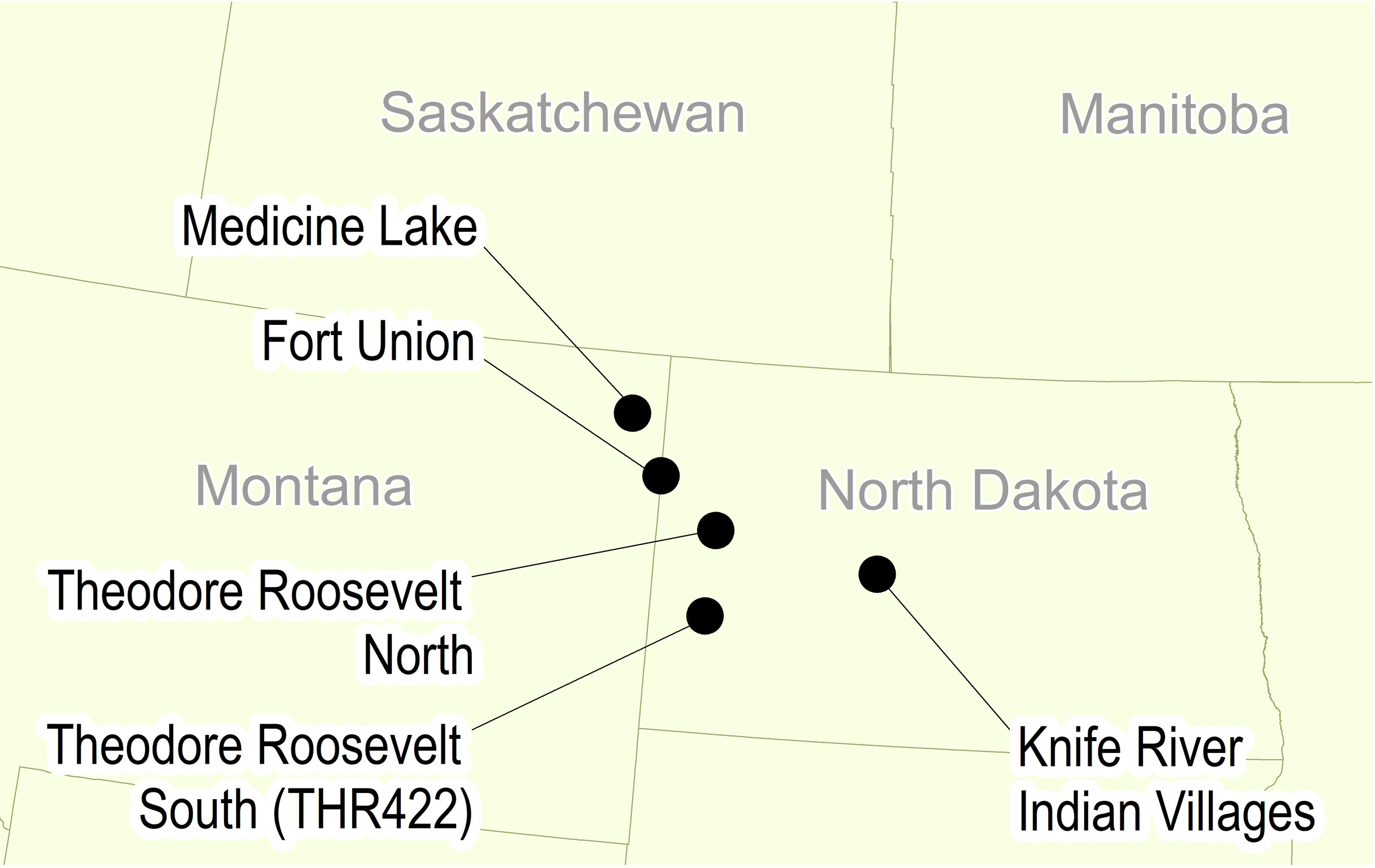
The rapid expansion of the oil and gas sector in the Bakken formation has the potential to impact three national park units in this region: Fort Union Trading Post (FOUS) National Historic Site (NHS), Knife River Indian Villages NHS (KNRI), and Theodore Roosevelt National Park (THRO), all located just miles from active oil and gas development. CASTNET operates THR422, ND in the south unit of THRO. FOUS and KNRI are Class II airsheds, while THRO is classified as a Class I airshed.
Class I airsheds are provided with the highest level of federal protection of air quality. There are also two U.S. Fish and Wildlife Service Class I areas nearby: Lostwood, ND and Medicine Lake, MT (MELA). At all of these sensitive areas, increased pollution can lead to a number of air quality issues, including exceedances of the NAAQS, contravention of goals of the Regional Haze Rule, and increased acid and reactive nitrogen deposition causing unwanted ecosystem changes.
Figure 4-f Number of Active Oil and Gas Wells in North Dakota and the Bakken Formation of North Dakota
 Download Figure
Source: https://www.dmr.nd.gov/oilgas/stats/statisticsvw.asp.
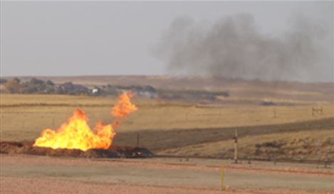
Source: NPS
Growing concern about potential impacts of oil and gas development on air quality in these natural areas prompted NPS to sponsor a special study in 2013–2014. The objectives of this study were to provide initial information on the composition and properties of particulate and gaseous pollutants in the national park units in the region and at Medicine Lake National Wildlife Refuge. Continuation of long-term monitoring in the THRO north unit is also being explored to track the changes in air quality over time.
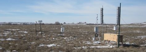
The first measurement period was a pilot study in February through April 2013. These dates coincide with typical maximum SO42- and NO3- concentrations measured at the THRO south unit as determined by the IMPROVE network. The study was conducted at five field sites (Figure 4-h), including the north and south units of THRO, FOUS, KNRI, and MELA. The north unit of THRO served as the core sampling site, while the satellite sites were intended to provide a regional assessment of air quality. MELA, located near the Canadian border and northwest of the THRO north unit, was included to assess potential contributions from the Canadian oil sands region. All sites included instruments to measure PM2.5 and its composition, trace gases, wet deposition, and meteorological conditions. Because the THRO south unit is already heavily instrumented through state and federal monitoring programs, only minimal sampling was conducted at this site. The THRO north core site contained an additional suite of continuous monitors to make measurements at higher time resolution and to measure particle scattering and trace gas concentrations. In addition to the fixed sampling sites, two days of measurements of methane and VOC were made using a mobile laboratory. Elevated methane concentrations throughout the study area suggested regional impacts from oil and gas activities.
During the pilot study, data from the high-time resolution measurements at the THRO north core site showed elevated concentrations of black carbon and PM2.5 precursors (NOx and SO2) throughout the campaign, with NOx and SO2 concentrations often exceeding 20 µg/m 3 and 10 µg/m 3, respectively. Consistent with these data were observations of elevated PM2.5 mass concentrations, both at the core and satellite sites. During one such episode, 24-hour average mass concentrations were over 14 µg/m 3, with the majority of the mass in the form of NH4NO3 and (NH4)2SO4. High mass concentrations and haze were typically associated with more stagnant air that recirculated throughout the Bakken study region, giving local emissions of precursor gases sufficient time to accumulate and react.
Observations of these particle episodes motivated a more in-depth study, which occurred November 2013 through March 2014. In addition to the maximum SO42- and NO3- concentrations expected during this time period, these dates encompass the largest increasing trends in SO42- and NO3- as determined from the IMPROVE network. During the second study, measurements were limited to three sites: the THRO north unit remained the core site while FOUS and MELA served as the satellite sites. At the THRO north unit and FOUS, additional measurements of gas and particle concentrations and compositions, most at high-time resolution, were made to better understand the processes that drive the high particle episodes. In addition, speciated VOC measurements were made twice a day at the core site, four times per week at FOUS, and once per week at MELA. These VOC data provide markers for many of the potential air pollutant sources in this region. Data from the second study are currently being analyzed to better characterize the processes that cause visibility impairment from aerosols in the region. As part of the ongoing data analysis efforts, receptor modeling will be conducted to qualitatively and semi-quantitatively assess the contributions of source regions and types to air quality at THRO.
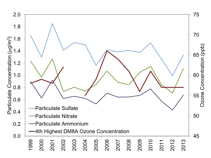
CASTNET measurements of O3 and particulate SO42-, NO3-, and NH4+ concentrations at THR422 supplement the air quality measurements taken by NPS in the Bakken region. Figure 4i illustrates trends in annual fourth highest DM8A O3 concentrations and 3-month mean February through April particulate SO42-, NO3-, and NH4+ concentrations from 1999 through 2013. The particulate measurements show downward trends in the three species. The O3 data show no trend in 3-year average fourth highest DM8A concentrations from 1999–2001 through 2011–2013.
Total Nitrate Concentrations
A map of 2013 mean total NO3- concentrations is provided in Figure 4-6. Figure 4-7 provides box plots of total NO3- levels for the eastern and western reference sites through 2013. The data shown on the right side of the figure were aggregated from the 34 eastern reference sites. The data show no trend in mean concentrations until 2000 when total NO3- levels began to decline in response to NOx emission control programs. Three-year mean levels declined from 3.0 µg/m 3 in 1990–1992 to 1.8 µg/m 3 in 2011–2013, producing a 41 percent reduction in total NO3-. Total NO3- levels measured at the eastern reference sites declined from a mean value of 3.1 µg/m 3 in 2000 to a mean value of 1.6 µg/m 3 in 2013.
The left side of Figure 4-7 shows data aggregated from the 17 western sites. The 3-year mean total NO3- concentration for 2011–2013 was 27 percent lower than the corresponding 1996–1998 level with 3-year mean concentrations of 0.7 µg/m 3 and 1.0 µg/m 3, respectively.
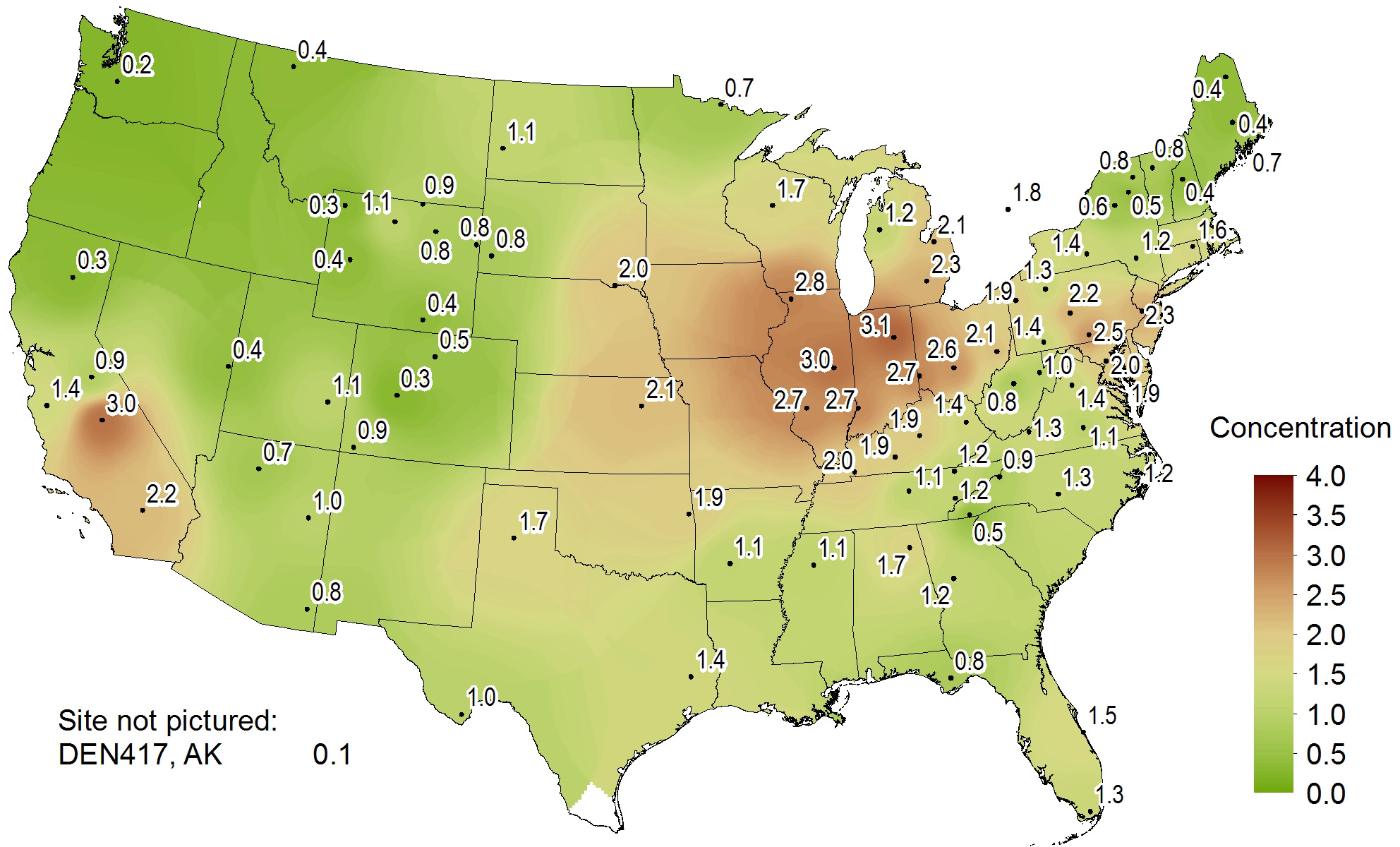
Total nitrate concentrations measured at the 34 eastern sites declined by about 41 percent. Total nitrate levels measured at the western reference sites were reduced by 27 percent. Total nitrate concentrations measured at the eastern sites were two to three times higher than concentrations measured at western reference sites.
Figure 4-7 Trends in Annual Mean Total NO3- Concentrations
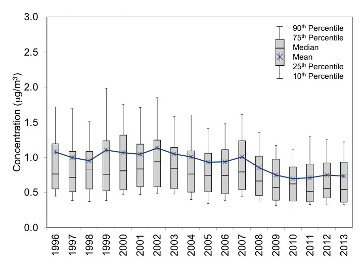
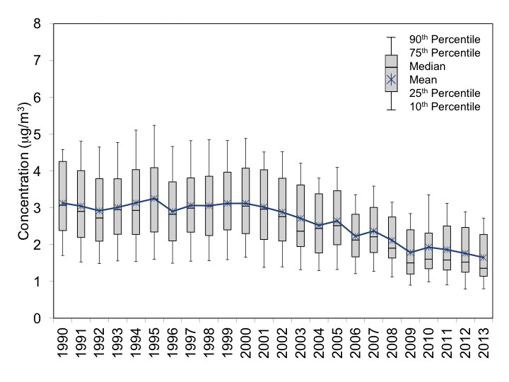
Figure 4-8 illustrates the trend in NOx emissions from regulated EGUs from 1990 through 2013 aggregated over six states (Illinois, Indiana, Kentucky, Ohio, West Virginia, and Pennsylvania). The 24-year decline in aggregated 6-state emissions was 78 percent.
Figure 4-8 Trend in Annual Composite NOx Emissions from Regulated EGUs Operating in Illinois, Indiana, Kentucky, Ohio, West Virginia, and Pennsylvania
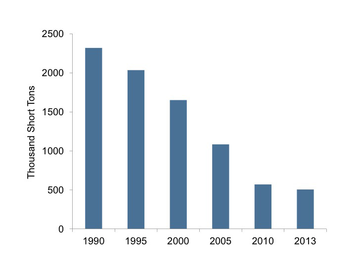 Download Figure
Note: Data from 415 EGUs in 1995, 518 in 2000, 751 in 2005, 747 in 2010, and 687 in 2013 were used to construct the bar chart.
Particulate Ammonium Concentrations
A map of 2013 mean particulate NH4+ concentrations is provided in Figure 4-9. Figure 4 10 shows box plots of NH4+ concentrations. The trend diagram for the eastern sites (right side) shows a reduction in mean NH4+ levels from 1990–1992 to 2011–2013. The 1990–1992 mean concentration was 1.8 µg/m 3, and the 2011–2013 value was 0.9 µg/m 3, a 50 percent decline.
The box plots characterizing the western sites (left side) show about a 17 percent reduction from 1996–1998 to 2010–2012 with 3-year mean concentrations declining from 0.3 µg/m 3 to 0.2 µg/m 3.
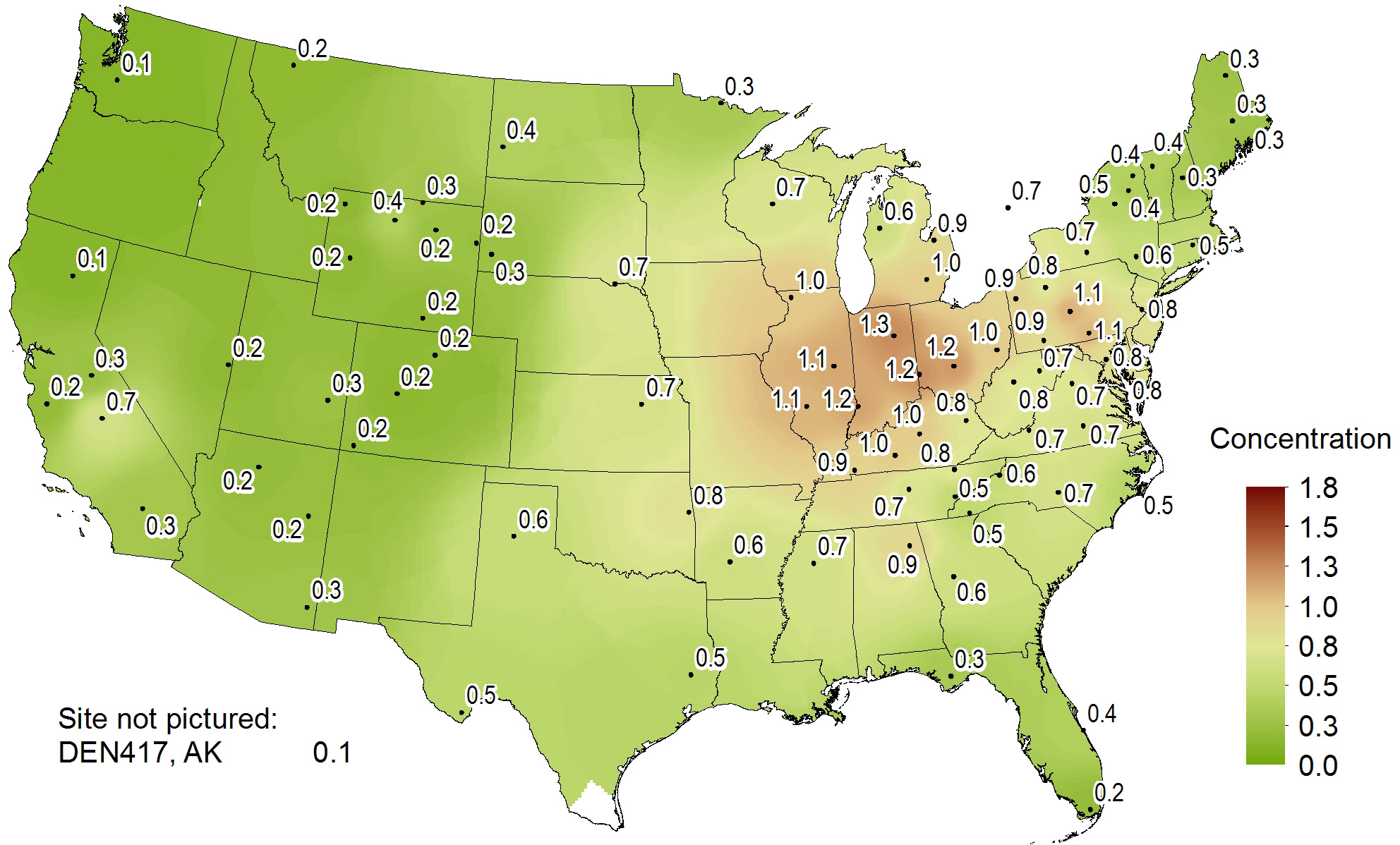
Figure 4-10 Trends in Annual Mean NH4+ Concentrations
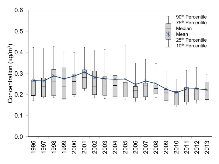
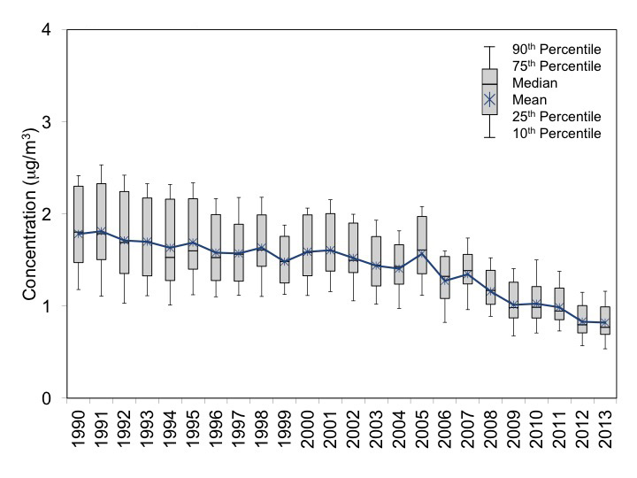
Table 4-1 summarizes the changes in sulfur and nitrogen pollutant concentrations aggregated over the western and eastern reference sites.
Table 4-1 Trends in Aggregated Western and Eastern Sulfur and Nitrogen Pollutant Concentrations
| Pollutant (µg/m 3) | Western Sites | Eastern Sites | Percent Changes | |||
|---|---|---|---|---|---|---|
| 1996-90 | 2011-13 | 1990-92 | 2011-13 | West | East | |
| SO2 | 0.6 | 0.3 | 8.9 | 1.7 | -54 | -80 |
| SO42- | 0.8 | 0.6 | 5.4 | 2.2 | -20 | -59 |
| Total NO3- | 1.0 | 0.7 | 3.0 | 1.8 | -27 | -41 |
| NH4+ | 0.3 | 0.2 | 1.8 | 0.9 | -17 | -50 |
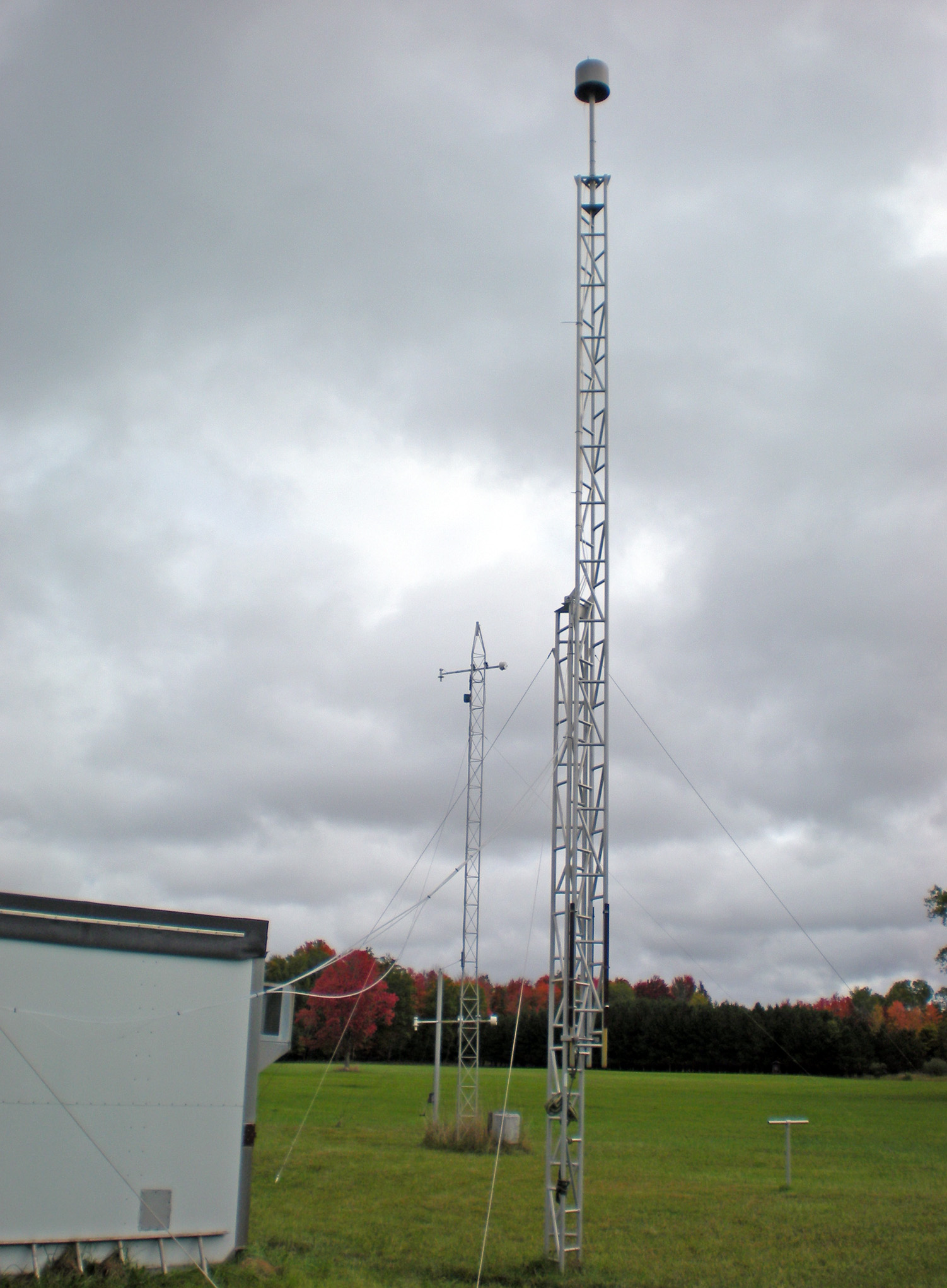
Hoxeyville, MI (HOX148)
Results for 2013 Environment Canada Proficiency Testing
During 2013, the AMEC CASTNET laboratory participated in the Environment Canada (ECAN) Proficiency Testing Program for Inorganic Environmental Substances. Specifically, the laboratory is one of 33 laboratories that participated in the 2013 Rain and Soft Waters round robin studies, which consist of natural waters supplied by the National Laboratory for Environmental Testing. The CASTNET laboratory receives 10 samples of mixed rain and Canadian Shield waters for chemical analysis from ECAN every six months. The laboratory reported the eight CASTNET parameters for samples in two studies (study codes 0102 and 0103) during 2013.
The results reported by the 33 laboratories are evaluated for systematic bias and precision. Systematic bias is assessed using Youden (1969) non-parametric analysis, while precision is calculated using algorithm A from the International Organization for Standardization (ISO) standard 13528 (ISO, 2005).
Individual sample results are flagged based on the Robust Standard Deviation (R-σ) obtained from the ISO 13528 computation (ISO, 2005). Samples within 2 standard deviations of the assigned (median laboratory) value are not flagged; samples between 2 and 3 standard deviations are given a warning flag; and samples greater than 3 standard deviations from the assigned value are flagged as above the action limit (remedial action is required). Laboratory results are considered systematically biased when individual parameters are ranked by the Youden analysis to be consistently and significantly higher or lower than the assigned value without regard to flagged results.
The CASTNET laboratory’s 2013 ECAN results for the eight CASTNET parameters are presented in Table 4-b. All eight parameters received the highest possible rating of “Ideal” indicating an unbiased score in study 0102. One of the 10 individual results for potassium was flagged “warning low” for study 0103, indicating that the flagged result was between 2 and 3 R-σ from its assigned value. Investigation by the laboratory revealed the root cause was an error in data processing. The data review process was revised for reporting future ECAN study results.
Table 4-b AMEC Results for Studies 0102 and 0103
| Test Parameter | Analytical Method | Reference Method | Laboratory Performance Rating | |
|---|---|---|---|---|
| Study 0102
Submitted July 2013 |
Study 0103
Submitted December 2013 |
|||
| Ammonia | AC | EPA Method 350.1 | Ideal | Ideal |
| Calcium | ICP-OES | EPA Method 6010 | Ideal | Ideal |
| Chloride | IC | EPA Method 300.0 | Ideal | Ideal |
| Magnesium | ICP-OES | EPA Method 6010 | Ideal | Ideal |
| Nitrate + Nitrite | IC | EPA Method 300.0 | Ideal | Ideal |
| Potassium | ICP-OES | EPA Method 6010 | Ideal | Ideal |
| Sodium | ICP-OES | EPA Method 6010 | Ideal | Ideal |
| Sulfate | IC | EPA Method 300.0 | Ideal | Ideal |
Note:
AC = automated colorimetry
ICP-OES = inductively coupled plasma - optical emission spectrometry
IC = ion chromatography
The overall laboratory performance rating was “Very Good” for both studies. The five-year historical laboratory rating for the AMEC CASTNET laboratory is listed by ECAN as “Very Good.”
Source: Environment Canada (2014)
Chapter 5: Atmospheric Deposition
CASTNET was designed to provide estimates of the dry deposition of sulfur and nitrogen pollutants across the United States. To assess the status of dry and total deposition for 2013, CASTNET used NADP’s Total Deposition Hybrid Method (TDEP) to estimate dry deposition by combining measured pollutant concentrations with output from the Community Multiscale Air Quality modeling system. TDEP used precipitation chemistry measurements at NADP/NTN sites and precipitation amounts from the Parameter-elevation Regressions on Independent Slopes Model (PRISM) to estimate wet deposition. Total deposition was calculated as the sum of estimated dry and wet deposition. Trends in deposition were estimated using the Multi-Layer Model (MLM)/Bowker/PRISM approach. Three-year mean total sulfur fluxes aggregated over the eastern reference sites declined by 66 percent over the period from 1990–1992 to 2011–2013. Three-year mean total sulfur deposition estimated for the 17 western reference sites declined by 39 percent over the period 1996–1998 to 2011–2013. Estimates of total nitrogen deposition declined 24 percent for the eastern reference sites and 18 percent at the western reference sites. In 2013, total sulfur and nitrogen deposition estimates were at or near historic lows.
Gaseous and particulate nitrogen and sulfur pollutants are deposited to the environment through dry and wet atmospheric processes. A principal goal of CASTNET is to estimate the rate of dry deposition from the atmosphere to sensitive ecosystems. NADP’s TDEP (EPA, 2014f; Schwede and Lear, 2014) combines monitoring data with output from the Community Multiscale Air Quality (CMAQ) modeling system (Byun and Schere, 2006). Air quality measurements are obtained from CASTNET, AMoN, and the Southeastern Aerosol Research and Characterization (SEARCH) Network. The TDEP method gives priority to measurement data from air quality monitoring sites when available and to CMAQ output in areas where monitoring data are not available. In addition, CMAQ provides modeled data for species that are not routinely measured. The TDEP method and its recent updates are discussed on the TDEP website. See also the NADP Fact Sheet, “Hybrid Approach to Mapping Total Deposition,”.
TDEP estimates wet deposition using PRISM to develop a continuous grid of precipitation data. PRISM uses terrain elevation, slope, and aspect and climatic measurements to estimate precipitation on a 4-kilometer resolution grid. For this report, pollutant concentrations in precipitation, which were estimated for the PRISM grid, were provided by NADP/NTN. The concentration and precipitation grids were merged in order to estimate pollutant wet deposition rates. Wet deposition rates for CASTNET sites were estimated from the four nearest grid cell values. Dry and wet deposition fluxes were added to obtain estimates of total deposition, which are presented on the maps as kilograms per hectare per year (kg/ha/yr).
Because TDEP is a dynamic product that is updated as new monitoring and modeling data become available, TDEP results were not used to estimate trends in deposition. Instead, the MLM/Bowker/PRISM approach that was used in previous CASTNET annual reports was used to project trends in dry and total deposition. The callout beginning on page 59 presents the results.
Sulfur Deposition
Figure 5-1 shows a map of TDEP-modeled dry sulfur (S) fluxes for 2013. The magnitude of the deposition fluxes is illustrated by the shading in the figure legend. A map of total S deposition is provided in Figure 5-2. The percentage of total S deposition due to dry S deposition is shown in Figure 5-3.
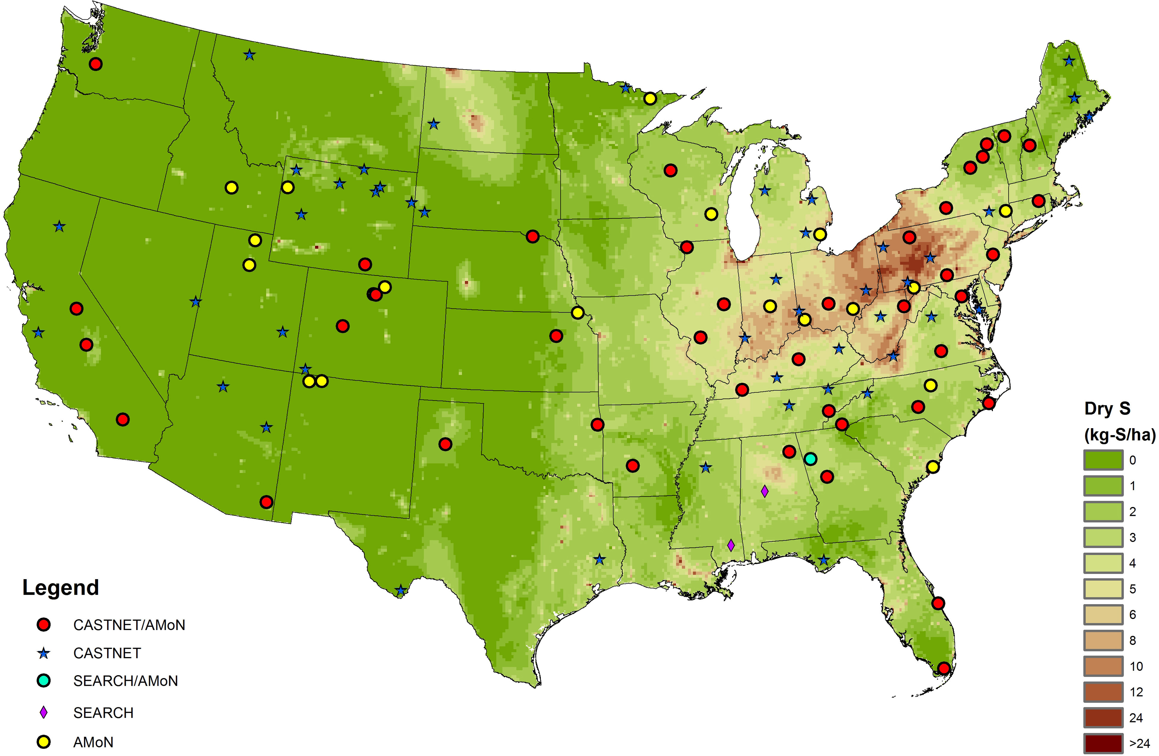
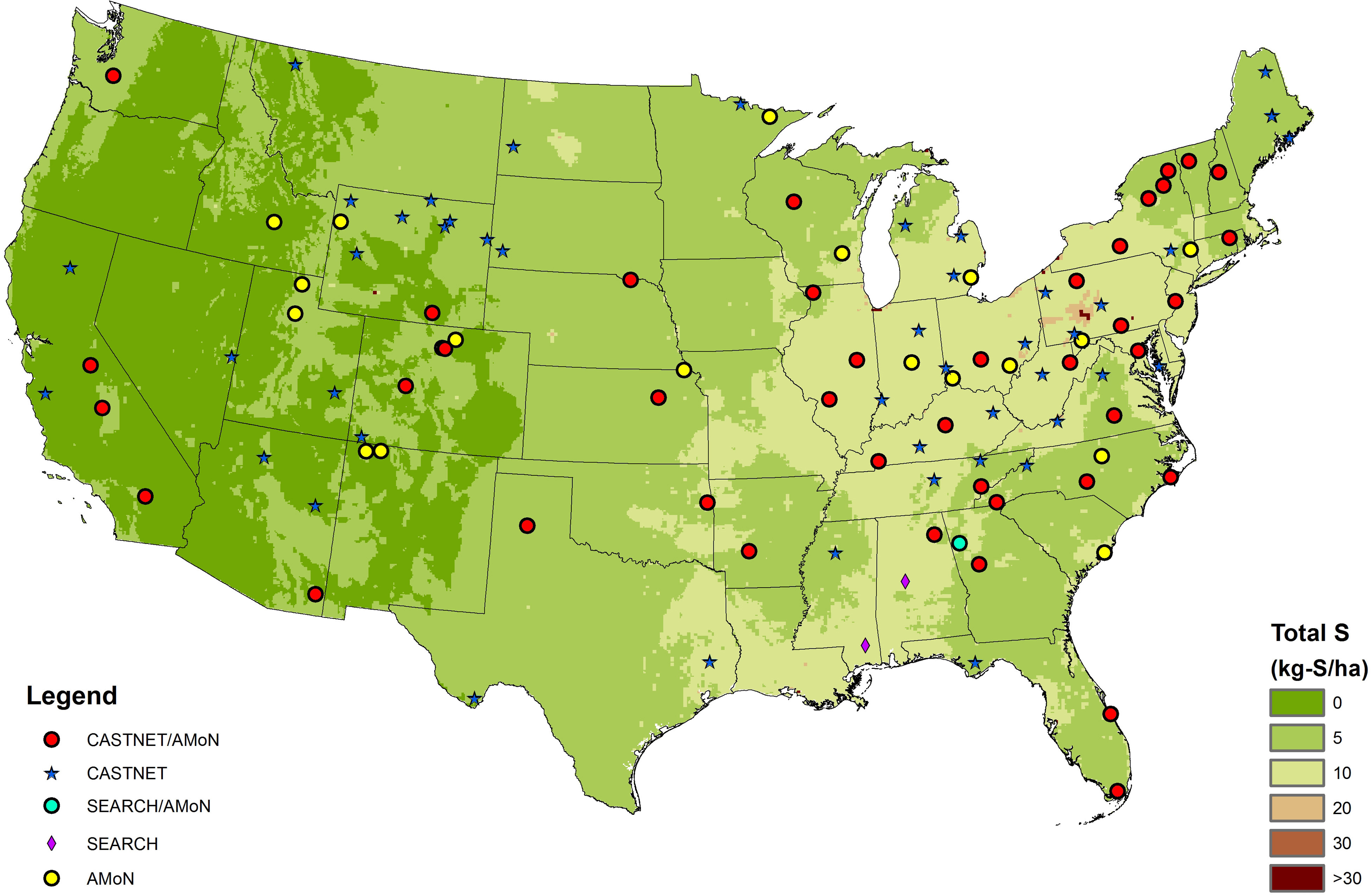
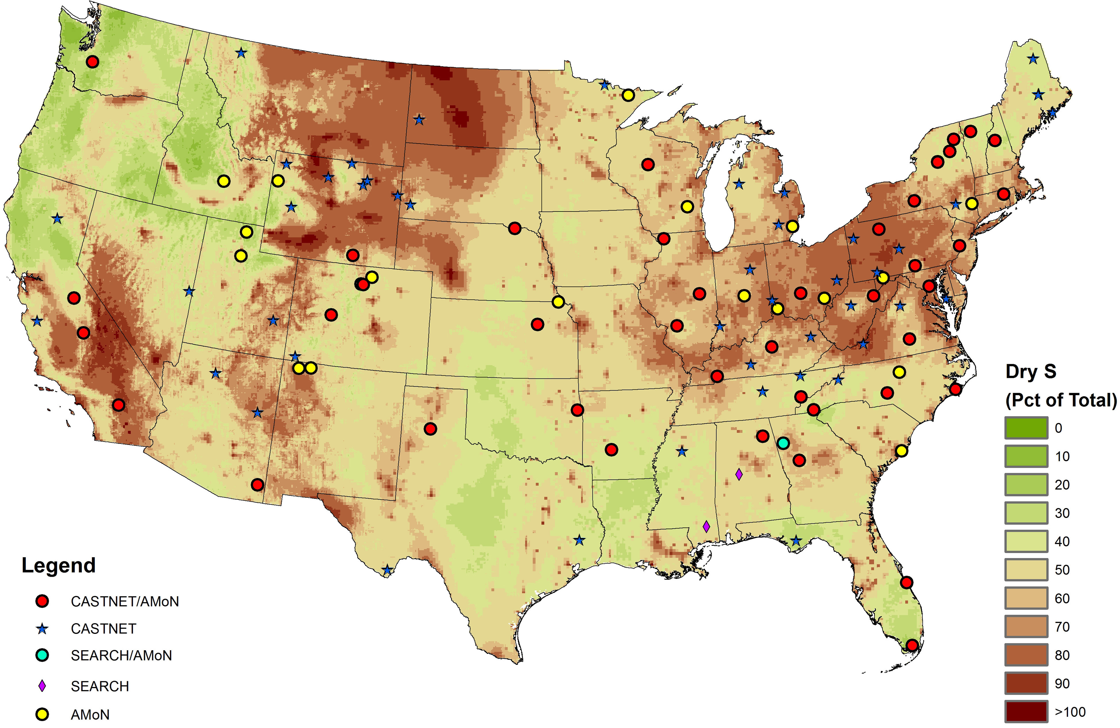
The Application and Use of Critical Loads for USDA Forest Service Management and Policy Decisions
The National Forest Management Act of 1976 (USDA, as amended) requires every national forest and grassland managed by the U.S. Department of Agriculture (USDA) Forest Service to develop and maintain a land management plan. The process for plan development and revision, along with the required plan content, is outlined in the Forest Service Planning Rule (USDA, 2012). The Forest Service released a revised planning rule in 2012 that, for the first time, requires national forests and grasslands to consider air quality when developing plan components. Specifically, planning rule directives require an assessment of critical loads (CL) and any CL exceedances (Nilsson and Grennfelt, 1988). If critical loads have been exceeded, managers of forests and grasslands are required to develop plan components to protect or restore key ecosystem characteristics.
These requirements provided a unique opportunity to standardize the way national forests view and manage air quality, specifically implementing the use of CL into the land management planning process. The Forest Service developed the Air Quality Portal for Land Management Planning in response to these new requirements. The Air Quality Portal is a decision support system based in large part on the CL information calculated and compiled by the NADP Critical Loads of Atmospheric Deposition Science Committee in the National Critical Loads Database. The Air Quality Portal incorporates CL information into land management by helping managers determine where atmospheric deposition is negatively affecting forest ecosystems and how to start the process of mitigation and/or restoration based on this information.
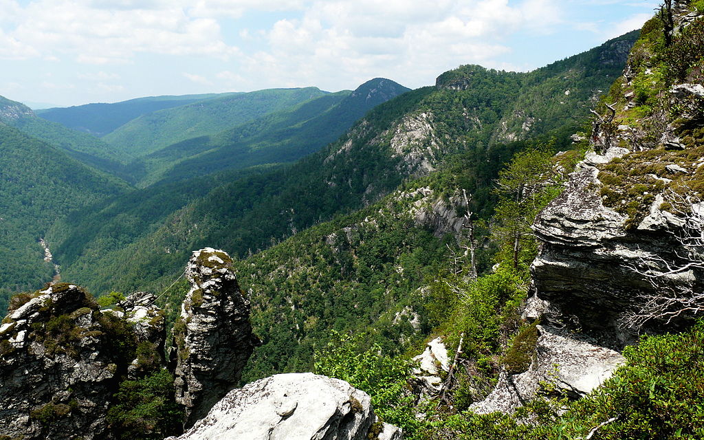
Linville Gorge Wilderness in the Pisgah National Forest
The Forest Service created an easy-to-use resource to guide national forest managers for considering and treating air quality for land management planning. The guide provides a nationally consistent method that incorporates the best available scientific data to help ensure the easing of the air pollution burden on our national forests. The portal site includes background information on atmospheric deposition and CL of air pollution, a standardized air quality assessment process (including guidance on assessing CL for land management planning), national air quality data, sample forest plan components and assessments, and training materials.
- Screen initial CL data for potential exceedances.
- Determine crucial concerns regarding the ecosystem, e.g., acidification or nitrogen saturation/eutrophication.
- Examine and analyze all available data, e.g., air quality, deposition, and CL estimates.
- Review the CL for forest(s) of concern.
- Identify the appropriate deposition information, e.g., 3-year average TDEP deposition estimates, to compare with CL, and calculate any exceedances.
- Examine critical exceedance patterns across the forest to better understand the extent and severity of potential impacts and assess the reliability of the CL exceedance information. CL exceedance metrics and how to use them are available on the portal.
- Analyze and interpret the CL exceedance and related information. Management recommendations will vary with the reliability and certainty of the CL exceedance estimates.
The portal recommends a 7-step implementation strategy:
The information developed through the seven steps will allow the formulation of a target load strategy. Target loads represent a policy or management decision about the amount of deposition that is an acceptable level for resource protection. Target loads for surface waters generally have a high level of certainty because they are estimated from reliable water chemistry measurements. On the other hand, estimates of CL for forested ecosystems are less certain because they are typically based on geospatially interpolated data that are not site specific. Currently, CL estimates for forested ecosystems are usually used to prepare a monitoring plan to generate site specific water chemistry, soil chemistry, and/or lichens data to improve estimates of target loads. Target load and monitoring strategies are discussed on the portal. Examples of descriptions of air quality, atmospheric pollutant deposition, and CL and target loads for Pisgah and Nantahala National Forests can be viewed on the website.
Source:USDA Forest Service (O’Dea and Huber, 2014)
Upper Creek Falls near the Community of Linville in Pisgah National Forest
Nitrogen Deposition
Figure 5-4 illustrates TDEP estimates of dry fluxes of nitrogen (as N) for 2013. The magnitude of the deposition fluxes is illustrated by the shading in the figure legend. A map of total N deposition for 2013 is given in Figure 5-5. The percentage of total N deposition due to dry N deposition is shown in Figure 5-6.
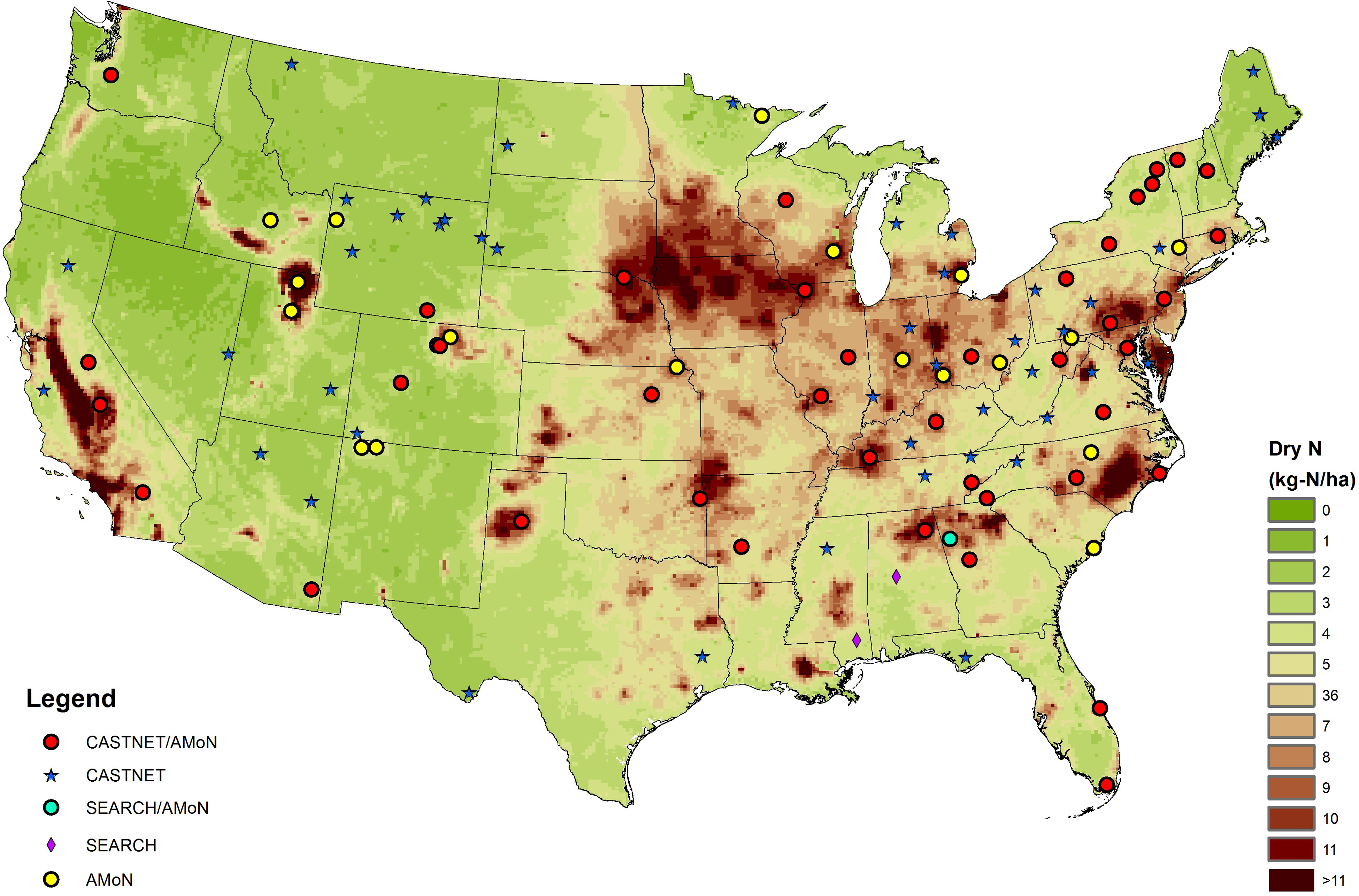
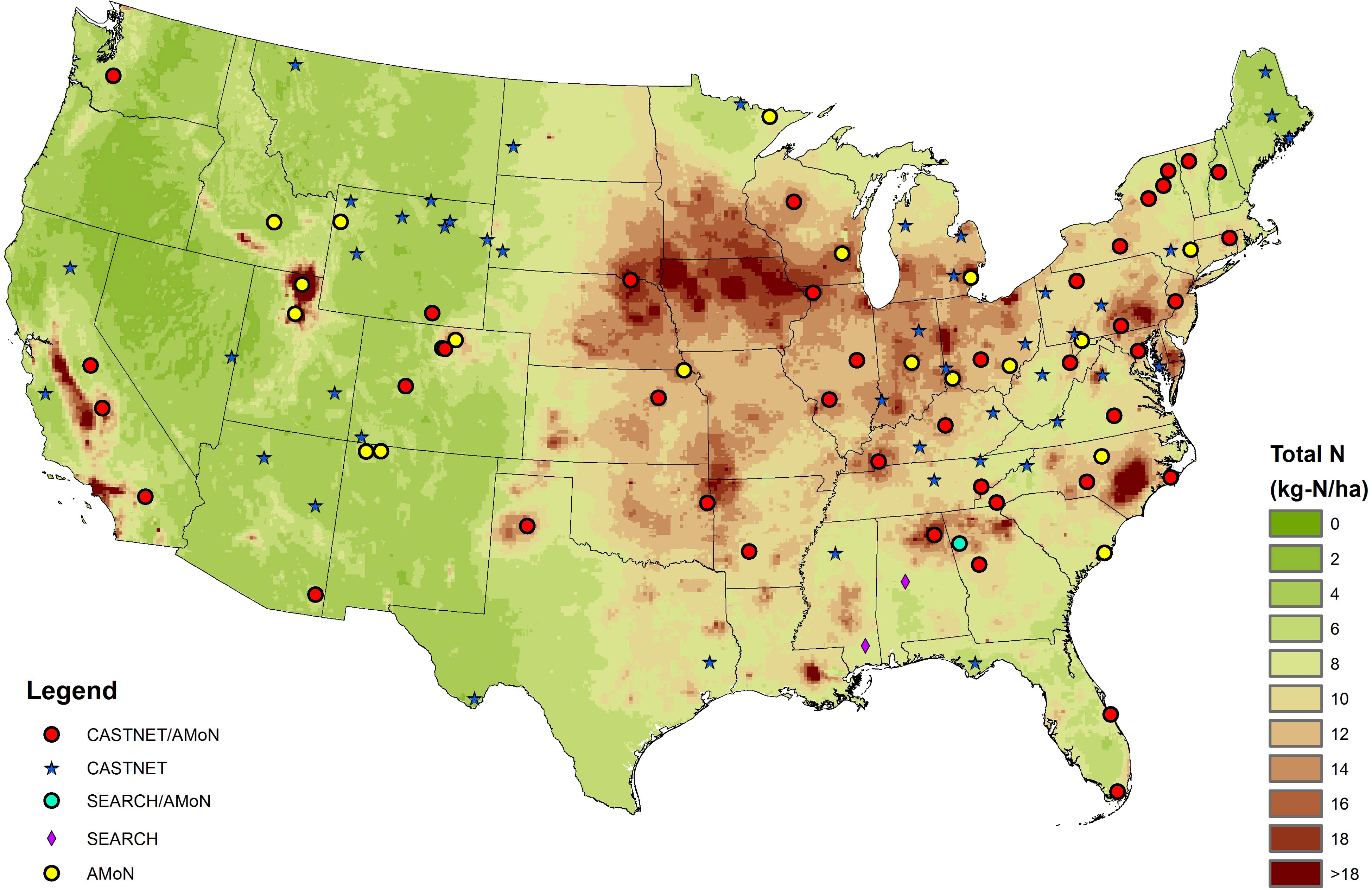
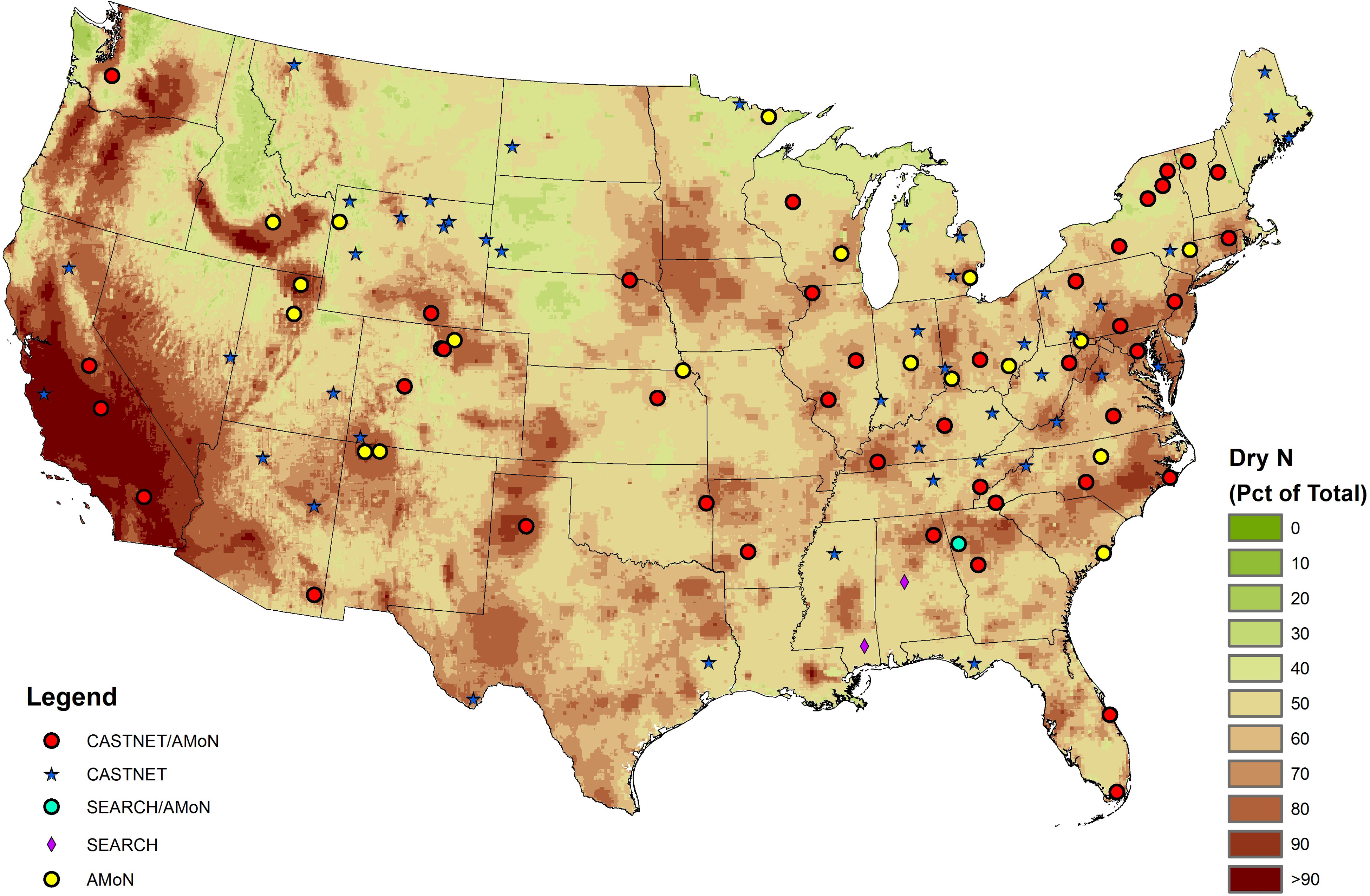
MLM/Bowker/PRISM Estimates of Trends in Dry and Total Sulfur and Nitrogen Deposition
The MLM/Bowker/PRISM approach (Bowker et al., 2011) that was used in previous CASTNET annual reports was used in this report to estimate trends in dry and total deposition. TDEP is a dynamic product that is updated at least annually as new monitoring and modeling data become available. Consequently, TDEP results are not comparable on an annual basis. As a result, in order to estimate trends, the MLM/Bowker/PRISM approach was applied instead. Table 5-a summarizes trends in dry and total deposition estimates for the western and eastern reference sites.
Table 5-a Trends in Aggregated Western and Eastern Sulfur and Nitrogen Pollutant Deposition Estimates
| Pollutant (kg/ha/yr) | Western Sites | Eastern Sites | Percent Changed | |||
|---|---|---|---|---|---|---|
| 1996-98 | 2011-13 | 1990-92 | 2011-13 | West | East | |
| Dry S | 0.3 | 0.2 | 5.1 | 1.1 | -40 | -78 |
| Total S | 1.3 | 0.8 | 12.9 | 4.3 | -39 | -66 |
| Dry N | 0.9 | 0.6 | 2.2 | 1.1 | -35 | -51 |
| Total N | 2.5 | 2.1 | 7.5 | 5.7 | -18 | -24 |
Trends in Sulfur Deposition
Box plots that show the trends in estimates of dry sulfur deposition (as S) for the eastern (right side) and western (left side) reference sites are provided in Figure 5-a. The box plots were based on data obtained from the 34 CASTNET eastern reference sites for the period 1990 through 2013 and from the 17 western reference sites for 1996 through 2013 (see Appendix A for reference site locations). The y axes on the two figures have different scales. Aggregated dry S deposition declined considerably at the eastern and western reference sites over their respective periods. Overall, dry S deposition declined at the eastern reference sites by 78 percent. Dry S deposition at the western reference sites showed a 40 percent reduction.
Figure 5-b shows the trends in estimates of annual total (dry + wet) sulfur deposition (as S) based on measurements taken at the CASTNET reference sites. Aggregated S deposition declined considerably at the eastern and western reference sites over their respective periods. Overall, total S deposition declined at the eastern sites by 66 percent. Total S deposition at the western reference sites was reduced 39 percent. The 2013 total S deposition estimates for eastern and western sites were the lowest in history of network. The relative contributions of dry and wet S deposition are shown in Figure 5-3.
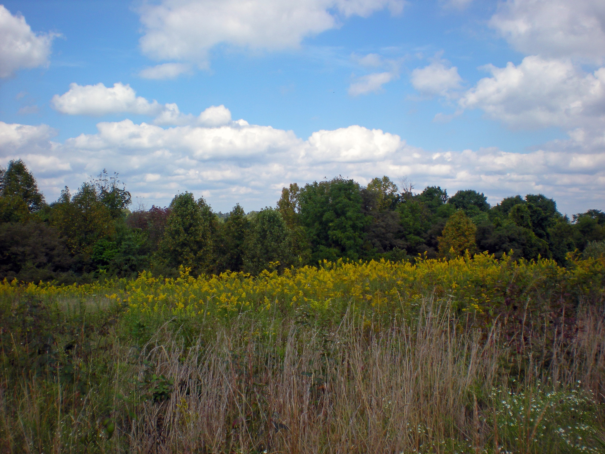
Scenic view from Quaker City, OH (QAK172)
Figure 5-a Trends in Dry S Deposition
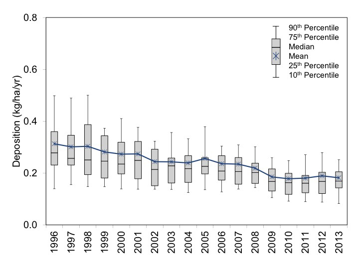
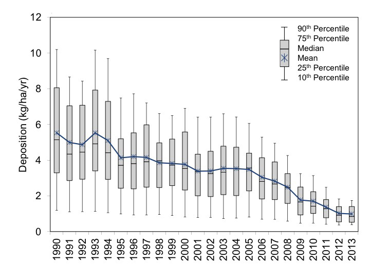
Figure 5-b Trends in Total S Deposition
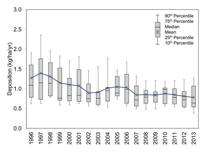
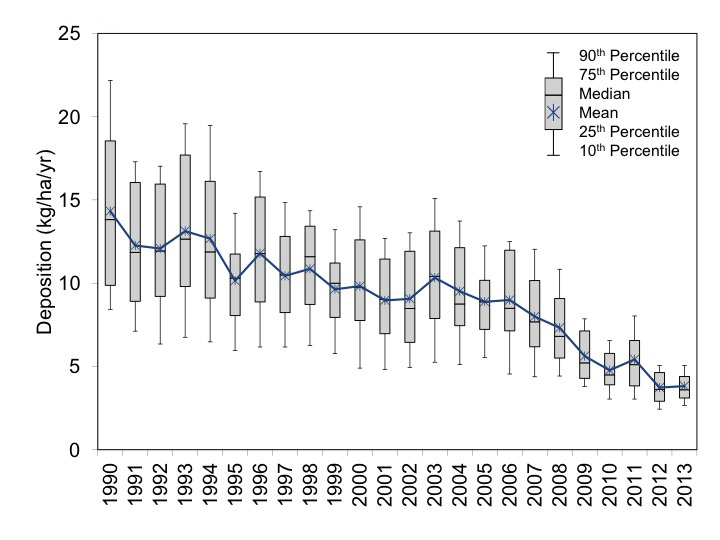
Trends in Nitrogen Deposition
Figure 5-c presents box plots that were constructed using data from the 34 CASTNET eastern reference sites over the period 1990 through 2013 (right side) and 17 western reference sites for 1996 through 2013 (left side). The box plots show the trends in estimates of dry nitrogen deposition (as N). The box plots in Figure 5-c for the eastern sites show a significant reduction in estimates of dry N deposition beginning in 2002. Three-year mean fluxes showed a 51 percent reduction over the 24 years. The box plots for the western sites show a 35 percent decline.
Figure 5-c Trends in Dry N Deposition
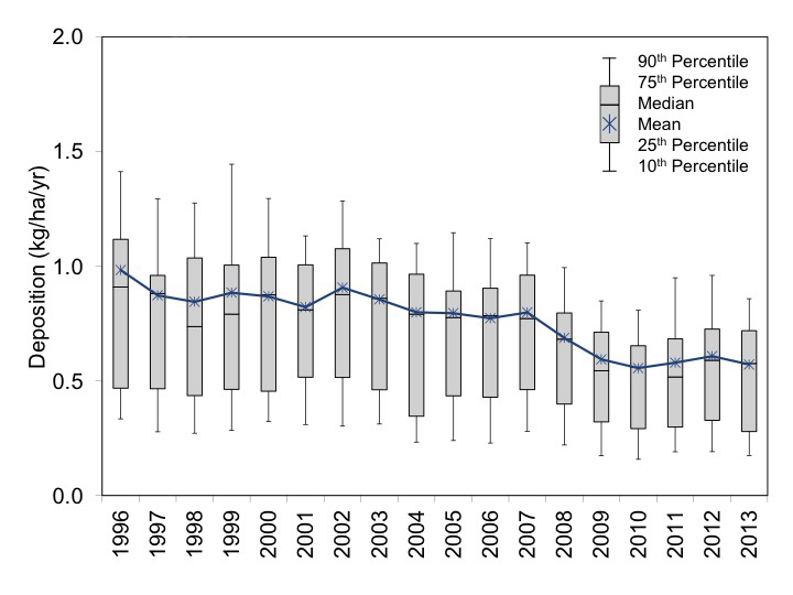
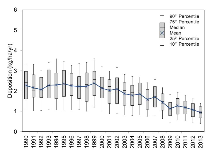
Figure 5-d depicts the trends in estimates of annual total (dry + wet) nitrogen deposition for the eastern (right side) and western (left side) reference sites. The figure shows that total nitrogen flux estimated for the eastern United States decreased since 1996 with a substantial decline from 2002 through 2010, an increase in 2011, and a subsequent decline through 2013. The median total nitrogen flux (5.2 kg/ha/yr) estimated for 2013 was the lowest ever measured. Total nitrogen deposition estimated for the eastern sites over the period 1990–1992 to 2011–2013 was reduced by 24 percent. Total nitrogen deposition estimated for the western sites shows a relatively flat trend from 1996–1998 to 2011–2013 with an 18 percent decline.
Figure 5-d Trends in Total N Deposition
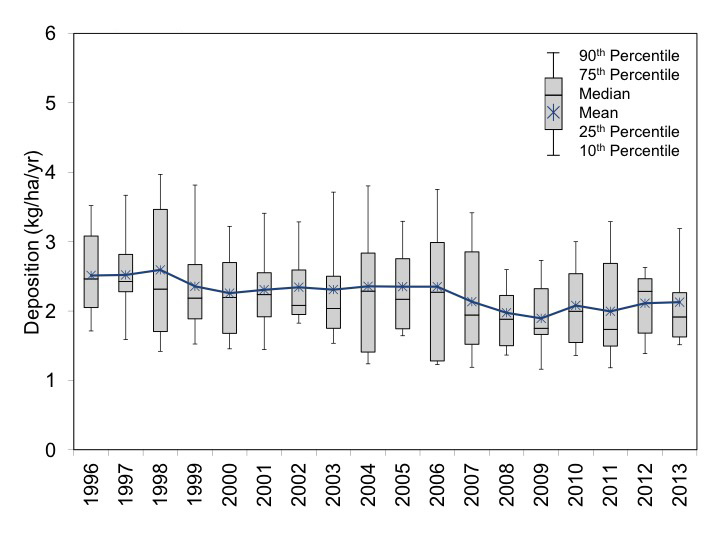
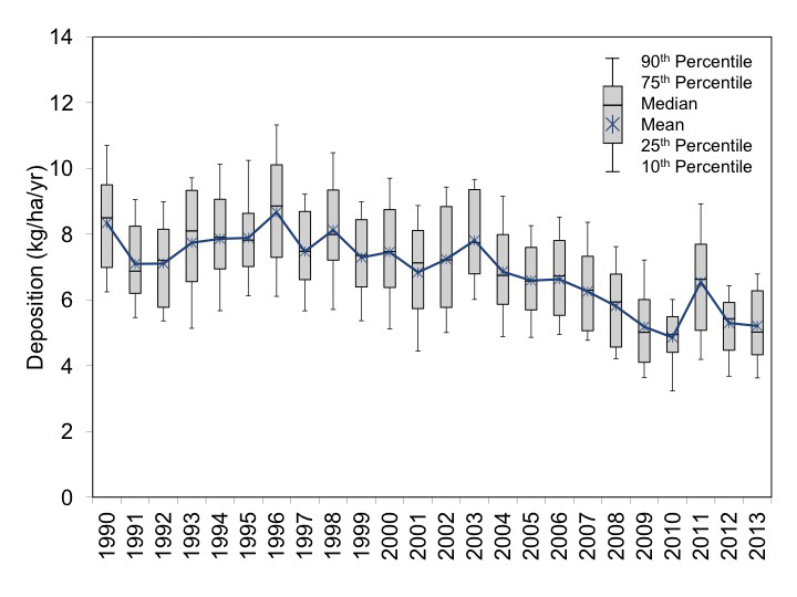
References
AMEC Environment & Infrastructure, Inc. (AMEC). 2014a. Clean Air Status and Trends Network (CASTNET) First Quarter 2014 Data Report. Prepared for U.S. Environmental Protection Agency (EPA), Office of Air and Radiation, Clean Air Markets Division, Washington, DC. Contract No. EP-W-09-028. Gainesville, FL.
AMEC Environment & Infrastructure, Inc. (AMEC). 2014b. Clean Air Status and Trends Network (CASTNET) Fourth Quarter 2013 Data Report. Prepared for U.S. Environmental Protection Agency (EPA), Office of Air and Radiation, Clean Air Markets Division, Washington, DC. Contract No. EP-W-09-028. Gainesville, FL.
AMEC Environment & Infrastructure, Inc. (AMEC). 2014c. Clean Air Status and Trends Network (CASTNET) Second Quarter 2014 Data Report. Prepared for U.S. Environmental Protection Agency (EPA), Office of Air and Radiation, Clean Air Markets Division, Washington, DC. Contract No. EP-W-09-028. Gainesville, FL.
AMEC Environment & Infrastructure, Inc. (AMEC). 2014d. Clean Air Status and Trends Network (CASTNET) Third Quarter 2013 Data Report. Prepared for U.S. Environmental Protection Agency (EPA), Office of Air and Radiation, Clean Air Markets Division, Washington, DC. Contract No. EP-W-09-028. Gainesville, FL.
AMEC Environment & Infrastructure, Inc. (AMEC). 2013a. Clean Air Status and Trends Network (CASTNET) 2011 Annual Report. Prepared for U.S. Environmental Protection Agency (EPA), Office of Air and Radiation, Clean Air Markets Division, Washington, DC. Contract No. EP-W-09-028. Gainesville, FL.
AMEC Environment & Infrastructure, Inc. (AMEC). 2013b. Clean Air Status and Trends Network (CASTNET) First Quarter 2013 Data Report. Prepared for U.S. Environmental Protection Agency (EPA), Office of Air and Radiation, Clean Air Markets Division, Washington, DC. Contract No. EP-W-09-028. Gainesville, FL.
AMEC Environment & Infrastructure, Inc. (AMEC). 2013c. Clean Air Status and Trends Network (CASTNET) Quality Assurance Project Plan (QAPP) Revision 8.1. Prepared for U.S. Environmental Protection Agency (EPA), Office of Air and Radiation, Clean Air Markets Division, Washington, DC. Contract No. EP-W-09-028. Gainesville, FL. http://java.epa.gov/castnet/documents.do.
AMEC Environment & Infrastructure, Inc. (AMEC). 2013d. Clean Air Status and Trends Network (CASTNET) Second Quarter 2013 Data Report. Prepared for U.S. Environmental Protection Agency (EPA), Office of Air and Radiation, Clean Air Markets Division, Washington, DC. Contract No. EP-W-09-028. Gainesville, FL.
AMEC Environment & Infrastructure, Inc. (AMEC). 2012. Clean Air Status and Trends Network (CASTNET) Quality Assurance Project Plan (QAPP) Revision 8.0. Prepared for U.S. Environmental Protection Agency (EPA), Office of Air and Radiation, Clean Air Markets Division, Washington, DC. Contract No. EP-W-09-028. Gainesville, FL. http://java.epa.gov/castnet/documents.do.
AMEC Environment & Infrastructure, Inc. (AMEC). 2003. Clean Air Status and Trends Network (CASTNET) 2002 Annual Report. Prepared for U.S. Environmental Protection Agency (EPA), Research Triangle Park, NC. Contract No. 68-D-03-052. Gainesville, FL.
Baumgardner, R.E., Rogers, C.M., Puchalski, M.R., Lavery, T.F., Mishoe, K.P., Price, G.L., and Hall, N.H. 2014. Measurements of Atmospheric NH 3, NOy/NOx, and NO2 and Deposition of Total Nitrogen at the Beaufort, NC CASTNET Site (BFT142). U.S. Environmental Protection Agency Office of Research and Development, Research Triangle Park, NC 27711. EPA/600-R-14/182.
Bowker, G.E., Schwede, D.B., Lear, G.G., Warren-Hicks, W.J., and Finkelstein, P.L. 2011. Quality Assurance Decisions with Air Models: A Case Study of Imputation of Missing Input Data Using EPA’s Multi-Layer Model. Water, Air, & Soil Pollution 223:391-402. DOI 10.1007/s11270-011-0832-7.
Byun, D. and Schere, K.L. 2006. Review of the Governing Equations, Computational Algorithms, and Other Components of the Models‐3 Community Multiscale Air Quality (CMAQ) Modeling System. Applied Mechanics Reviews, 59: 51‐77. DOI 10.1115/1.2128636.
Environment Canada (ECAN) Water Science and Technology Directorate. 2014. Rain and Soft Waters PT Studies 0102 and 0103 Report. Proficiency Testing Program, Burlington, Ontario, Canada. Prepared for AMEC Environment & Infrastructure, Inc.
Hand, J.L., Schichtel, B.A., Malm, W.C., Copeland, S., Molenar, J.V., Frank, N., and Pitchford, M. 2014. Widespread Reductions in Haze across the United States from the Early 1990s through 2011, Atmos. Environ., 94:671-679. DOI: 10.1016/j.atmosenv.2014.05.062
International Organization for Standardization (ISO). 2005. Statistical Methods for the Use in Proficiency Testing by Interlaboratory Comparisons, Annex C, Robust Analysis, Section C.1: Algorithm A. Standard 13528. ISO 13528:2005(E).
Lefohn, A.S. and Runeckles, V.C. 1987. Establishing a Standard to Protect Vegetation - Ozone Exposure/Dose Considerations. Atmos. Environ., 21:561-568.
National Crop Loss Assessment Network (NCLAN). 2013. Ozone and Crop Plants, http://people.oregonstate.edu/~muirp/ozeffect.htm (accessed December 2013)
Nilsson, J., and Grennfelt, P. (Eds). 1988. Critical Loads for Sulphur and Nitrogen. UNECE/Nordic Council workshop report, Skokloster, Sweden. March 1988. Nordic Council of Ministers: Copenhagen.
North Dakota Oil and Gas Division. 2015. North Dakota Industrial Commission Order 24665 Policy/Guidance. https://www.dmr.nd.gov/oilgas/GuidancePolicyNorthDakotaIndustrialCommissionorder24665.pdf. Accessed May 2015.
O’Dea, C. and Huber, C. 2014. Development and Release of the Air Quality Portal for Land Management Planning: The Application and Use of Critical Loads for Management and Policy Decisions. http://nadp.sws.uiuc.edu/conf/2014/abstract.aspx?abstractID=39. Accessed December 2014.
Puchalski, M.A, Sather, M.E., Walker, J.T., Lehmann, C.M.B., Gay, D.A., Mathew, J., and Robarge, W.P. 2011. Passive Ammonia Monitoring in the United States: Comparing Three Different Sampling Devices. J. Environ. Monit., 13:3156-67. DOI: 10.1039/c1em10553a
Schwede, D.B. and Lear, G.G. 2014. A Novel Hybrid Approach for Estimating Total Deposition in the United States. Atmos. Environ., 92:207-220. DOI: 10.1016/j.atmosenv.2014.04.008.
Talbot, R., Mao, H., and Sive, B. 2005. Diurnal Characteristics of Surface Level O 3 and other Important Trace Gases in New England, J. Geophys. Res., 110, D09307, doi:10.1029/2004JD005449.
U.S. Department of Agriculture (USDA) Forest Service. 2012. National Forest System Land Management Planning; Final Rule. Federal Register 77, No. 68 (April 9), http://www.fs.usda.gov/Internet/FSE_DOCUMENTS/stelprdb5362536.pdf. Accessed March 2015.
U.S. Department of Agriculture (USDA) Forest Service. The National Forest Management Act of 1976. 16 USC Section 1600–1687 (as amended). http://www.fs.fed.us/emc/nfma/includes/RPA_amended_by_NFMA_USCover.pdf.
U.S. Environmental Protection Agency (EPA). 2014a. Availability of Data on Allocations of Cross-State Air Pollution Rule Allowances to Existing Electricity Generating Units. http://www.epa.gov/crossstaterule/pdfs/CSAPRallocationsNODA11_12_14.pdf. Accessed December 2014.
U.S. Environmental Protection Agency (EPA). 2014b. Overview of EPA’s Proposal to Update the Air Quality Standards for Ground-Level Ozone. http://www.epa.gov/glo/pdfs/20141125fs-overview.pdf. Accessed December 2014.
U.S. Environmental Protection Agency (EPA). 2014c. Proposed Rule by the Environmental Protection Agency to the National Ambient Air Quality Standards for Ozone. 79 Federal Register 75233. https://www.federalregister.gov/articles/2014/12/17/2014-28674/national-ambient-air-quality-standards-for-ozone Accessed December 2014.
U.S. Environmental Protection Agency (EPA). 2014d. Rulemaking to Amend Dates in Federal Implementation Plans Addressing Interstate Transport of Ozone and Fine Particulate Matter. http://www.epa.gov/crossstaterule/pdfs/CSAPRinterimfinal11_12_14.pdf. Accessed December 2014.
U.S. Environmental Protection Agency (EPA). 2014e. Supreme Court Reversed the D.C. Circuit Opinion Vacating CSAPR. http://www.epa.gov/airtransport/CSAPR/index.html. Accessed June 2014.
U.S. Environmental Protection Agency (EPA). 2014f. Total Deposition Estimates Using a Hybrid Approach. ftp://ftp.epa.gov/castnet/tdep/Total_Deposition_Documentation_2014v02.pdf. Accessed November 2014.
U.S. Environmental Protection Agency (EPA). 2013. Treatment of Data Influenced by Exceptional Events. http://www.epa.gov/ttn/analysis/exevents.htm. Accessed December 2014.
U.S. Environmental Protection Agency (EPA). 2010a. Appendix A to Part 58 – Quality Assurance Requirements for State and Local Air Monitoring Stations (SLAMS), Special Purpose Monitors (SPMs), and Prevention of Significant Deterioration (PSD) Air Monitoring. 40 CFR Part 58.
U.S. Environmental Protection Agency (EPA). 2010b. Proposed Revisions to National Standards for Ground-Level Ozone. http://www.epa.gov/air/ozonepollution/actions.html Accessed December 2014.
U.S. Environmental Protection Agency (EPA). 2008a. National Ambient Air Quality Standards for Ozone; Final Rule. Federal Register 73, No. 60 (March). EPA-HQ-OAR-2005-0172.
U.S. Environmental Protection Agency (EPA). 2008b. Quality Assurance Handbook for Air Pollution Measurement Systems, Volume II, Ambient Air Quality Monitoring Program. EPA-454/B-08-003, December.
U.S. Environmental Protection Agency (EPA). 2006. Air Quality Criteria for Ozone and Related Photochemical Oxidants. Report No. EPA/600/R-05/004af. ORD, Research Triangle Park, NC.
U.S. Environmental Protection Agency (EPA). 1998. Guideline on Data Handling Conventions for the 8-Hour Ozone NAAQS. EPA-454/R-98-017. OAQPS, Research Triangle Park, NC 27711.
U.S. Environmental Protection Agency (EPA). 1996. Air Quality Criteria for Ozone and Related Photochemical Oxidants. EPA Report No. EPA/600/P-93/004bF. ORD, Research Triangle Park, NC.
Youden, W.J. (Ku, H.H., ed). 1969. Precision Measurement and Calibration. NBS Special Publication 300-Volume 1. U.S. Government Printing Office, Washington, DC.
Appendix A: Locational and Operational Characteristics of CASTNET Sites
| Site ID | Site Name | Start Date | Latitude | Longitude | Elevation | Nearby NADP | Land Use | Terrain | Agency | Reference |
|---|---|---|---|---|---|---|---|---|---|---|
| ABT147, CT | Abington | 12/28/1993 | 41.8405 | -72.0104 | 202 | CT15 | Urban/Agric | Rolling | EPA | |
| ACA416, ME | Acadia NP | 12/1/1998 | 44.3771 | -68.2608 | 158 | ME98 | Forest | Rolling | NPS | |
| ALC188, TX | Alabama-Coushatta | 4/6/2004 | 30.7016 | -94.674 | 105 | TX10 | Prairie | Rolling | EPA | |
| ALH157, IL | Alhambra | 6/28/1988 | 38.869 | -89.6228 | 164 | IL46 | Agric | Flat | EPA | E |
| ANA115, MI | Ann Arbor | 6/28/1988 | 42.4166 | -83.9022 | 266 | MI52 | Forest | Flat | EPA | E |
| ARE128, PA | Arendtsville | 6/28/1988 | 39.9232 | -77.3079 | 266 | PA00 | Agric | Rolling | EPA | E |
| ASH135, ME | Ashland | 12/20/1988 | 46.6038 | -68.4132 | 231 | ME00 | Agric | Flat | EPA | E |
| BAS601, WY | Basin | 11/6/2012 | 44.28 | -108.0411 | 1242 | MT00 | Prairie | Rolling | BLM | |
| BBE401, TX | Big Bend NP | 7/18/1995 | 29.3027 | -103.1778 | 1052 | TX04 | Forest | Complex | NPS | W |
| BEL116, MD | Beltsville | 11/1/1988 | 39.0282 | -76.8171 | 47 | MD99 | Range | Flat | EPA | E |
| BFT142, NC | Beaufort | 12/28/1993 | 34.8847 | -76.6207 | 5 | NC06 | Agric | Flat | EPA | |
| BUF603, WY | Buffalo | 11/6/2012 | 44.1442 | -106.1089 | 1324 | WY99 | Prairie | Rolling | BLM | |
| BVL130, IL | Bondville | 2/9/1988 | 40.052 | -88.3725 | 213 | IL11 | Agric | Flat | EPA | E |
| BWR139, MD | Blackwater NWR | 7/4/1995 | 38.445 | -76.1113 | 1 | MD15 | Forest/Marsh | Coastal | EPA | |
| CAD150, AR | Caddo Valley | 10/4/1988 | 34.1793 | -93.0988 | 78 | AR03 | Forest | Complex | EPA | E |
| CAN407, UT | Canyonlands NP | 1/24/1995 | 38.4583 | -109.8213 | 1809 | UT09 | Desert | Complex | NPS | W |
| CAT175, NY | Claryville | 5/10/1994 | 41.9423 | -74.552 | 754 | NY68 | Forest | Complex | EPA | |
| CDR119, WV | Cedar Creek | 11/10/1987 | 38.8795 | -80.8477 | 240 | WV05 | Forest | Complex | EPA | E |
| CDZ171, KY | Cadiz | 9/28/1993 | 36.7841 | -87.8502 | 190 | KY99 | Agric | Rolling | EPA | |
| CHA467, AZ | Chiricahua NM | 4/25/1989 | 32.0094 | -109.3891 | 1570 | AZ98 | Range | Complex | NPS | W |
| CHE185, OK | Cherokee Nation | 4/2/2002 | 35.7508 | -94.6698 | 305 | AR27 | Agric | Rolling | EPA | |
| CKT136, KY | Crockett | 8/24/1993 | 37.9215 | -83.0663 | 376 | KY35 | Agric | Rolling | EPA | |
| CND125, NC | Candor | 9/25/1990 | 35.2633 | -79.8375 | 172 | NC36 | Forest | Rolling | EPA | E |
| CNT169, WY | Centennial | 5/9/1989 | 41.3645 | -106.24 | 3175 | WY95 | Forest | Complex | EPA | W |
| COW137, NC | Coweeta | 11/4/1987 | 35.0605 | -83.4303 | 683 | NC25 | Forest | Complex | EPA | E |
| CTH110, NY | Connecticut Hill | 9/29/1987 | 42.4009 | -76.6535 | 511 | NY67 | Forest | Rolling | EPA | E |
| CVL151, MS | Coffeeville | 12/27/1988 | 34.0027 | -89.7992 | 138 | MS30 | Forest | Rolling | EPA | |
| DCP114, OH | Deer Creek | 9/28/1988 | 39.6359 | -83.2606 | 264 | OH54 | Agric | Rolling | EPA | E |
| DEN417, AK | Denali NP | 10/6/1998 | 63.7232 | -148.9676 | 661 | AK03 | Forest | Complex | NPS | |
| DIN431, UT | Dinosaur NM | 11/20/2013 | 40.4373 | -109.3046 | 1463 | CO15 | Desert | Complex | NPS | |
| EGB181, ON | Egbert | 12/27/1994 | 44.2311 | -79.7831 | 227 | NY10 | Agric | Rolling | EPA | |
| ESP127, TN | Edgar Evins | 3/22/1988 | 36.0389 | -85.7331 | 302 | KY10 | Forest | Rolling | EPA | E |
| EVE419, FL | Everglades NP | 10/6/1998 | 25.3912 | -80.6808 | 2 | FL11 | Forest/Marsh | Flat | NPS | |
| FOR605, WY | Fortification Creek | 5/21/2013 | 44.3395 | -105.9198 | 1408 | WY99 | Prairie | Rolling | BLM | |
| GAS153, GA | Georgia Station | 6/28/1988 | 33.1812 | -84.4101 | 265 | GA41 | Agric | Rolling | EPA | E |
| GLR468, MT | Glacier NP | 12/27/1988 | 48.5103 | -113.9968 | 976 | MT05 | Forest | Complex | NPS | W |
| GRB411, NV | Great Basin NP | 5/16/1995 | 39.0051 | -114.2159 | 2060 | NV05 | Forest | Complex | NPS | W |
| GRC474, AZ | >Grand Canyon NP | 5/16/1989 | 36.0586 | -112.1836 | 2073 | AZ03 | Forest | Rolling | NPS | W |
| GRS420, TN | Great Smoky Mountains NP - Look Rock | 10/16/1998 | 35.6335 | -83.9416 | 793 | TN11 | Forest | Complex | NPS | |
| GTH161, CO | Gothic | 5/16/1989 | 38.9563 | -106.9859 | 2915 | CO10 | Range | Complex | EPA | W |
| HOW191, ME | Howland Ameriflux | 9/27/2011 | 45.204 | -68.74 | 68 | ME09 | Forest | Rolling | EPA | |
| HOX148, MI | Hoxeyville | 10/31/2000 | 44.1809 | -85.739 | 297 | MI53 | Forest | Flat | EPA | |
| HWF187, NY | Huntington Wildlife Forest | 5/28/2002 | 43.973 | -74.2233 | 497 | NY20 | Forest | Complex | EPA | |
| IRL141, FL | Indian River Lagoon | 7/9/2001 | 27.8492 | -80.4556 | 2 | FL99 | Coastal/Marsh | Flat/Water | EPA | |
| JOT403, CA | Joshua Tree NP | 2/16/1995 | 34.0696 | -116.3889 | 1244 | CA67 | Desert | Complex | NPS | W |
| KEF112, PA | Kane Experimental Forest | 1/3/1989 | 41.5981 | -78.7679 | 618 | PA29 | Forest | Rolling | EPA | E |
| KNZ184, KS | Konza Prairie | 3/26/2002 | 39.1022 | -96.6096 | 346 | KS31 | Prairie | Flat | EPA | |
| LAV410, CA | Lassen Volcanic NP | 7/25/1995 | 40.54 | -121.5765 | 1756 | CA96 | Forest | Complex | NPS | W |
| LRL117, PA | Laurel Hill | 12/15/1987 | 39.9883 | -79.2516 | 609 | MD08 | Forest | Complex | EPA | E |
| MAC426, KY | Mammoth Cave NP | 7/24/2002 | 37.1318 | -86.143 | 243 | KY10 | Agric | Rolling | NPS | |
| MCK131, KY | Mackville | 7/31/1990 | 37.7047 | -85.0487 | 293 | KY03 | Agric | Rolling | EPA | E |
| MCK231, KY | Mackville Collocated | 12/29/1992 | 37.7047 | -85.0487 | 293 | KY03 | Agric | Rolling | EPA | |
| MEV405, CO | Mesa Verde NP | 1/10/1995 | 37.1984 | -108.4905 | 2165 | CO99 | Forest | Complex | NPS | W |
| MKG113, PA | M.K. Goddard | 1/12/1988 | 41.4268 | -80.1452 | 377 | NY10 | Forest | Rolling | EPA | E |
| MOR409, WA | Mount Rainier NP | 8/29/1995 | 46.7584 | -122.1243 | 415 | WA99 | Forest | Complex | NPS | W |
| NEC602, WY | Newcastle | 11/7/2012 | 43.873 | -104.1919 | 1468 | WY99 | Prairie | Rolling | BLM | |
| NIC001, NY | Nicks Lake | 11/20/2012 | 43.6805 | -74.9891 | 525 | NY29 | Forest | Rolling | NYSDEC | |
| OXF122, OH | Oxford | 8/18/1987 | 39.5311 | -84.7235 | 284 | OH09 | Agric | Rolling | EPA | E |
| PAL190, TX | Palo Duro Canyon SP | 4/24/2007 | 34.8806 | -101.6647 | 1053 | TX02 | Prairie | Complex | EPA | |
| PAR107, WV | Parsons | 1/19/1988 | 39.0904 | -79.6617 | 510 | WV18 | Forest | Complex | EPA | E |
| PED108, VA | Prince Edward | 11/3/1987 | 37.1652 | -78.3071 | 149 | VA24 | Forest | Rolling | EPA | E |
| PET427, AZ | Petrified Forest NP | 9/12/2002 | 34.8225 | -109.8925 | 1723 | AZ97 | Desert | Flat | NPS | |
| PIN414, CA | Pinnacles NM | 5/16/1995 | 36.4832 | -121.1569 | 335 | CA66 | Forest | Complex | NPS | W |
| PND165, WY | Pinedale | 12/27/1988 | 42.929 | -109.7878 | 2386 | WY06 | Forest | Rolling | EPA | W |
| PNF126, NC | Cranberry | 12/27/1988 | 36.1054 | -82.045 | 1216 | NC45 | Forest | Mountaintop | EPA | E |
| PRK134, WI | Perkinstown | 9/27/1988 | 45.2065 | -90.5972 | 462 | WI35 | Agric | Rolling | EPA | E |
| PSU106, PA | Penn State | 1/6/1987 | 40.7209 | -77.9318 | 364 | PA42 | Agric | Rolling | EPA | E |
| QAK172, OH | Quaker City | 9/28/1993 | 39.9427 | -81.3379 | 371 | OH49 | Agric | Rolling | EPA | |
| ROM206, CO | Rocky Mountain NP Collocated | 7/3/2001 | 40.2781 | -105.5456 | 2742 | CO19 | Forest | Complex | EPA | |
| ROM406, CO | Rocky Mountain NP | 12/20/1994 | 40.2781 | -105.5456 | 2743 | CO19 | Forest | Complex | NPS | W |
| SAL133, IN | Salamonie Reservoir | 6/28/1988 | 40.816 | -85.6614 | 250 | IN20 | Agric | Flat | EPA | E |
| SAN189, NE | Santee Sioux | 7/5/2006 | 42.8292 | -97.8541 | 434 | SD99 | Range | Rolling | EPA | |
| SEK430, CA | Sequoia NP - Ash Mountain | 4/7/2005 | 36.4895 | -118.8292 | 510 | CA75 | Forest | Mountaintop | NPS | |
| SHE604, WY | Sheridan | 11/6/2012 | 44.93 | -106.85 | 1115 | MT00 | Prairie | Rolling | BLM | |
| SHN418, VA | Shenandoah NP - Big Meadows | 6/28/1988 | 38.5231 | -78.4347 | 1073 | VA28 | Forest | Mountaintop | NPS | E |
| SND152, AL | Sand Mountain | 12/27/1988 | 34.289 | -85.9701 | 349 | AL99 | Agric | Rolling | EPA | E |
| SPD111, TN | Speedwell | 6/12/1989 | 36.4698 | -83.8265 | 361 | TN04 | Agric | Rolling | EPA | E |
| STK138, IL | Stockton | 12/28/1993 | 42.2872 | -90 | 281 | IL18 | Agric | Rolling | EPA | |
| SUM156, FL | Sumatra | 12/27/1988 | 30.1102 | -84.9904 | 16 | FL23 | Forest | Flat | EPA | E |
| THR422, ND | Theodore Roosevelt NP | 10/6/1998 | 46.8948 | -103.3777 | 850 | ND00 | Forest | Rolling | NPS | |
| UND002, VT | Underhill | 11/13/2012 | 44.5283 | -72.8688 | 399 | VT99 | Forest | Complex | EPA | |
| UVL124, MI | Unionville | 6/28/1988 | 43.6136 | -83.3599 | 202 | MI51 | Agric | Flat | EPA | E |
| VIN140, IN | Vincennes | 8/4/1987 | 38.7408 | -87.4849 | 136 | IN22 | Agric | Rolling | EPA | E |
| VOY413, MN | Voyageurs NP | 6/13/1996 | 48.4125 | -92.8292 | 429 | MN32 | Forest | Rolling | NPS | |
| VPI120, VA | Horton Station | 6/2/1987 | 37.3298 | -80.5575 | 920 | VA13 | Agric | Mountaintop | EPA | E |
| WFM105, NY | Whiteface Mountain | 11/20/2012 | 44.39 | -73.86 | 570 | NY98 | Forest | Complex | NYSERDA | |
| WNC429, SD | Wind Cave NP | 11/20/2003 | 43.5576 | -103.4839 | 1292 | SD04 | Prairie | Rolling | NPS | |
| WSP144, NJ | Wash. Crossing | 12/27/1988 | 40.3123 | -74.8727 | 59 | NJ99 | Range | Rolling | EPA | E |
| WST109, NH | Woodstock | 12/27/1988 | 43.9445 | -71.7008 | 255 | NH02 | Forest | Complex | EPA | E |
| YEL408, WY | Yellowstone NP | 6/26/1996 | 44.5654 | -110.4003 | 2400 | WY08 | Agric | Rolling | NPS | W |
| YOS404, CA | Yosemite NP - Turtleback Dome | 9/25/1995 | 37.7133 | -119.7062 | 1605 | CA99 | Forest | Complex | NPS | W |
Note:
NM = National Monument
NP = National Park
NWR = National Wildlife Reserve
SP = State Park
E = eastern reference site
W = western reference site
Appendix B: Acronyms and Abbreviations
| AAI | aquatic acidification index |
| ALPHA | Adapted Low-cost Passive High Absorption sampler |
| AMEC | AMEC Environment & Infrastructure, Inc. |
| AMNet | Atmospheric Mercury Network |
| AMoN | Ammonia Monitoring Network |
| AQS | EPA’s Air Quality System |
| ARP | Acid Rain Program |
| BLM | Bureau of Land Management |
| CAAA | Clean Air Act Amendments |
| CAIR | Clean Air Interstate Rule |
| CAPMoN | Canadian Air and Precipitation Monitoring Network |
| CASTNET | Clean Air Status and Trends Network |
| CFR | Code of Federal Regulations |
| CL | critical loads |
| Cl -- | particulate chloride ion |
| CMAQ | Community Multiscale Air Quality Modeling System |
| CO | carbon monoxide |
| CSAPR | Cross-State Air Pollution Rule |
| DM8A | daily maximum 8-hour average |
| DQI | data quality indicator |
| ECAN | Environment Canada |
| EGUs | electric generating units |
| EPA | U.S. Environmental Protection Agency |
| ESF | Environmental Science and Forestry |
| FOUS | Fort Union Trading Post |
| Hg | mercury |
| HNO3 | nitric acid |
| IMPROVE | Interagency Monitoring of Protected Visual Environments |
| ISO | International Organization for Standardization |
| kg/ha/yr | kilograms per hectare per year |
| km | kilometer |
| KNRI | Knife River Indian Villages |
| m | meter |
| MARPD | mean absolute relative percent difference |
| MELA | Medicine Lake, MT |
| MDN | Mercury Deposition Network |
| MLM | Multi-Layer Model |
| N | nitrogen |
| NAAQS | National Ambient Air Quality Standards |
| NADP | National Atmospheric Deposition Program |
| NBP | NOx Budget Trading Program |
| NCLAN | National Crop Loss Assessment Network |
| NCore | EPA’s National Core Monitoring |
| NH3 | ammonia |
| NH4+ | particulate ammonium |
| NH4NO3 | ammonium nitrate |
| NHS | National Historic Site |
| (NH4)2SO4 | ammonium sulfate |
| NO | nitrogen oxide |
| NO2 | nitrogen dioxide |
| NO3- | particulate nitrate |
| NOx | nitrogen oxides [nitrogen oxide (NO) + nitrogen dioxide (NO2)] |
| NOy | total reactive oxides of nitrogen |
| NOz | HNO3, nitrous oxide, peroxyacetyl nitrate, peroxyproyl nitrate, other organic nitrates, and nitrite |
| NPS | National Park Service |
| NTN | National Trends Network |
| NYSDEC | New York State Department of Environmental Conservation |
| O3 | ozone |
| OTC | Ozone Transport Commission |
| PM | particulate matter |
| PM2.5 | fine particulate matter |
| PRISM | Parameter-elevation Regressions on Independent Slopes Model |
| ppb | parts per billion |
| ppm | parts per million |
| QA | quality assurance |
| QAPP | Quality Assurance Project Plan |
| R-σ | robust standard deviation |
| RTD | resistance-temperature device |
| S | sulfur |
| SEARCH | Southeastern Aerosol Research and Characterization Network |
| SIP | State Implementation Plan |
| SO2 | sulfur dioxide |
| SO42- | particulate sulfate |
| STN | Speciation Trends Network |
| SOPs | standard operating procedures |
| SUNY | State University of New York |
| TDEP | NADP’s Total Deposition Hybrid Method |
| THRO | Theodore Roosevelt National Park |
| total NO3- | gaseous nitric acid (HNO 3) + particulate nitrate (NO- 3) |
| USDA | U.S. Department of Agriculture |
| µg/m&nbps;3 | micrograms per cubic meter |
| VOC | volatile organic compounds |
| WARMS | Wyoming Air Resources Monitoring System |