Executive Summary
The EPA Clean Air Status and Trends Network (CASTNET) monitors atmospheric pollutant concentrations across the United States. The primary objectives of the network are to determine compliance with ozone National Ambient Air Quality Standards and to provide data to evaluate the effectiveness of national and regional air pollution control programs. CASTNET data are also used to provide input to the National Atmospheric Deposition Program’s Total Deposition Hybrid Method for calculating total and dry deposition. This report presents maps of 2017 ozone levels, nitrogen and sulfur pollutant concentrations, and deposition fluxes. Additionally, it provides box plots to show trends in air quality over the 28-year period from 1990 through 2017. In 2017, CASTNET measured rural, regionally representative concentrations of nitrogen and sulfur species at 95 monitoring stations at 93 locations and ozone levels at 82 locations.
Key Results and Highlights through 2017
The median fourth highest daily maximum 8-hour average (DM8A) ozone (O3) concentration for 2017 at the eastern CASTNET reference sites (see Appendix A for designated reference sites) was 62 parts per billion (ppb). This is a decrease from the 2016 median of 65 ppb. At the western CASTNET reference sites, the median was 67 ppb, an increase from the 2016 value of 65 ppb. Three-year averages of fourth highest DM8A O3 concentrations exceeded the 2015 8-hour National Ambient Air Quality Standard (NAAQS) of 0.070 parts per million (ppm) or, equivalently, 70 ppb, at three CASTNET sites in California, one in New Jersey, one in Connecticut, and one in Utah during the most recent 3-year period (2015–2017). During 2017, fourth highest DM8A O3 concentrations greater than 70 ppb were observed at the same six CASTNET sites in California, New Jersey, Connecticut, and Utah that measured the highest concentrations in 2015-2017. Three-year averages of fourth highest DM8A O3 concentrations have been reduced by 24 percent at the eastern reference sites since 1990– 1992 and by 10 percent at the western reference sites since 1996–1998. Figure E-1 and Table E-1 summarize the long-term changes in measured concentrations.

Federal, state, and local NOx control programs have resulted in substantive reductions in emissions. NOx emissions declined by 89 percent over the 28-year period, 1990 through 2017, at regulated electric generating units (EGUs) in the East. Three-year mean annual concentrations of total nitrate (NO3-), which is comprised of nitric acid plus particulate NO3-, declined 51 percent at the eastern reference sites over the 28-year period. Three-year mean annual total NO3- levels measured at the western reference sites dropped by 37 percent over the 21-year period.
Mean annual sulfur dioxide (SO2) concentrations measured at the eastern reference sites have declined significantly over the 28-year period, 1990 through 2017. Three-year mean annual SO2 levels at eastern sites decreased 89 percent reflecting the reduction in regulated eastern EGU SO2 emissions (96 percent). SO2 concentrations measured at the western reference sites declined by 45 percent over the 21 years from 1996 through 2017.
| Pollutant | Western Reference Sites | Eastern Reference Sites | Percent Changed | |||
|---|---|---|---|---|---|---|
| 1996-1998 | 2014-2016 | 1990-1992 | 2014-2016 | West | East | |
| O3 (ppb) | 74 | 66 | 85 | 64 | -10 | -24 |
| Total NO3- (µg/m 3 ) | 1.0 | 0.6 | 3.0 | 1.5 | -37 | -51 |
| SO2 (µg/m 3 ) | 0.6 | 0.3 | 8.8 | 0.9 | -45 | -89 |
The original intent of CASTNET was to measure pollutant concentrations to estimate trends in sulfur and nitrogen pollutants. Currently, the focus also includes measuring rural, regional O3 concentrations. The network also features measurements of trace-level gases and speciated nitrogen pollutants. Additionally, CASTNET supports the National Atmospheric Deposition Program’s Ammonia Monitoring Network with operation of ammonia samplers at 65 CASTNET sites. This report provides information on CASTNET pollutant measurements, estimated deposition fluxes, and other topics that can be addressed using CASTNET data, such as the contribution of stratospheric O3 to ground-level concentrations in the Intermountain West and the effects of the California wildfires in October and December 2017 on air quality.
Chapter 1: CASTNET Update
The Clean Air Status and Trends Network (CASTNET) is a nationwide air quality monitoring network that began operating in 1991. The network provides long-term measurements of air pollutant concentrations in rural areas across the United States to determine compliance with ozone National Ambient Air Quality Standards and to evaluate the effectiveness of national and regional emission control programs. CASTNET data are used to provide input to regional air quality models in order to calculate atmospheric pollutant deposition. CASTNET is managed and operated by the U.S. Environmental Protection Agency in cooperation with the National Park Service and other federal, state, tribal, and local partners. In 2017, the network operated 96 monitoring stations throughout the contiguous United States, Alaska, and Canada. CASTNET data show a 28-year decline in ozone concentrations and in nitrogen and sulfur pollutant levels and deposition rates.
Introduction
The Clean Air Status and Trends Network (CASTNET) operated 96 monitoring stations throughout the contiguous United States, Alaska, and Canada in 2017. Ninety-five of 96 sites included filter pack systems to sample weekly concentrations of acid gases and aerosols. Eighty-two sites included continuous ozone (O3) analyzers. The U.S. Environmental Protection Agency (EPA) and the National Park Service (NPS) are the primary sponsors of CASTNET. NPS began its participation in 1994 and operated 26 sites during 2017. The Bureau of Land Management-Wyoming State Office (BLM) operated five sites in Wyoming.
CASTNET depends on contributions from many organizations (EPA, 2018a) including Native American tribes, state and federal government agencies, and universities. These participants sponsor individual CASTNET sites and provide in-kind services that support the overall performance of the network. For example, partners operate and repair site instruments, change weekly filter packs, and perform general site maintenance. Many partners provide the land for the CASTNET site. Others, such as universities, provide their expertise in air quality monitoring, which is invaluable for improving CASTNET monitoring capabilities and ensuring that CASTNET collects data that are of value to the scientific research community.
In 2017, ozone monitoring was initiated at Chaco Canyon, NM (CHC432). This site is the sole ozone-only CASTNET site in the network. It is the first CASTNET site in New Mexico. Filter pack sampling and an enhanced nitrogen oxide/total reactive oxides of nitrogen (NO/NOy) system, which permits speciation of reactive nitrogen components, began operating at Duke Forest, NC (DUK008). The seasonal small footprint site at the summit of Whiteface Mountain, NY (WFM007) was operated by the New York State Department of Environmental Conservation during the summer of 2017. Trace-level gas measurements were discontinued at Beltsville, MD (BEL116).
The U.S. Congress established the Acid Rain Program (ARP) in 1990 to reduce emissions of sulfur dioxide (SO2) and nitrogen oxides (NOx) from electric generating units (EGUs). CASTNET was created to assess the effectiveness of the ARP by providing consistent, long-term measurements for determining relationships between changes in emissions and changes in air quality, atmospheric deposition, and ecological effects..
Related Air Quality Networks
CASTNET monitors air quality and deposition in cooperation with other national and international networks. EPA uses data from CASTNET and the other long-term national networks to assess the effectiveness of emission control programs. These networks include the National Atmospheric Deposition Program (NADP; http://nadp.slh.wisc.edu/) and its affiliated networks:
- National Trends Network (NTN)
- Ammonia Monitoring Network (AMoN)
- Mercury Deposition Network (MDN)
- Atmospheric Mercury Network (AMNet)
Other cooperating networks include:
- Canadian Air and Precipitation Monitoring Network (CAPMoN)
- EPA’s National Core Monitoring (NCore)
- BLM’s Wyoming Air Resources Monitoring System (WARMS)
- Interagency Monitoring of Protected Visual Environments (IMPROVE)
Locations of Monitoring Sites
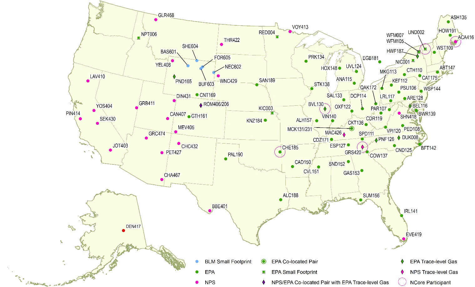
A map of CASTNET monitoring sites is given in Figure 1-1. Ninety-six monitoring sites were operated at 94 distinct locations. To estimate precision across the network, co-located sites were operated at Mackville, KY (MCK131/231) and Rocky Mountain National Park, CO (ROM406/206) during 2017. The ROM406/206 pair ensures consistency between EPA (ROM206) and NPS (ROM406). Of the two Rocky Mountain monitoring sites, ROM406 is specified as the regulatory monitoring site for O3. The location of each site and information on start date, latitude, longitude, elevation, identification of the nearby NADP site, land use, terrain type, operating agency, and if the site is a reference site used for trends are given in Appendix A.
Measurements Recorded at CASTNET Sites
During 2017, all but one CASTNET site measured weekly ambient concentrations of acidic pollutants, base cations, and chloride (Cl -) using a 3-stage filter pack with a controlled flow rate (Wood, 2017). Gaseous pollutant concentrations include nitric acid (HNO3) and SO2. Particulate concentrations include nitrate (NO3-), ammonium (NH4+), sulfate (SO42-), magnesium (Mg 2+ ), calcium (Ca 2+ ), potassium (K + ), sodium (Na + ), and Cl -. The filter pack is exchanged each Tuesday and shipped to the analytical chemistry laboratory for analysis. Ambient temperature is measured at 9 meters (m) at all sites in part to enable conversion of concentrations to local conditions.
Most CASTNET sites also include a temperature-controlled shelter and continuous O3 monitoring system. O3 concentrations were measured at 82 sites. The O3 inlet and filter pack are located atop a 10-m tower. Some CASTNET sites also measure trace-level SO2, carbon monoxide (CO), and NO/NOy. In 2017, meteorological parameters were measured at 6 EPA-, 26 NPS-, and 5 BLM-sponsored CASTNET sites. Measured meteorological parameters include 2-m temperature, wind speed and direction, standard deviation of the wind direction, solar radiation, relative humidity, precipitation, and surface wetness (at select sites).
Quality Assurance Program
The CASTNET quality assurance (QA) program was established to ensure that all reported data are of known and documented quality in order to meet CASTNET objectives. The QA program also ensures intranetwork consistency and comparability and the delivery of data that are reproducible and comparable with data from other monitoring networks. The 2017 QA program elements are documented in the CASTNET Quality Assurance Project Plan (QAPP; Wood, 2017). The QAPP includes standards and policies for all components of project operation, from site selection through final data reporting, with appendices that provide standard operating procedures for CASTNET operations.
Data quality indicators (DQI) such as precision, accuracy, and completeness are used to assess CASTNET measurements and supporting activities. Routine assessment and analysis help guarantee the production of high-quality data and information to meet project objectives. Measurements taken during 2017 and historical data collected over the period 1990 through 2016 were analyzed relative to DQI and their associated metrics. Results from these analyses are available in quarterly and annual QA reports posted on the EPA CASTNET website.
The Wood CASTNET laboratory regularly participates in interlaboratory comparison studies and proficiency testing (PT) programs such as the Environment Canada (ECAN) PT Program for Inorganic Environmental Substances. The ECAN PT program conforms to the requirements of the American Association for Laboratory Accreditation. The program meets the International Organization for Standardization (ISO)/International Electrotechnical Commission 17043:2010 conformity assessment – general requirements for proficiency testing with scope of accreditation 2867.01. The results reported are evaluated for systematic bias and precision. Systematic bias is assessed using the Youden (1969) non-parametric analysis, while precision is calculated using algorithm A from the ISO standard 13528 (ISO, 2005). CASTNET laboratory results from the PT studies are summarized in the QA annual reports posted to the EPA CASTNET website.
Estimating Dry, Wet, and Total Deposition
Total deposition was assessed using the NADP’s Total Deposition Hybrid Method (EPA, 2015c; Schwede and Lear, 2014), which is a hybrid approach that combines data from established ambient monitoring networks and chemical transport models. To estimate dry deposition, ambient concentration measurement data from CASTNET were merged with dry deposition flux output from the Community Multiscale Air Quality (CMAQ) modeling system. Wet deposition estimates were derived from precipitation chemistry measurements and precipitation amounts from the Parameter-elevation Regressions on Independent Slopes Model (PRISM). NADP-measured precipitation and chemistry data and precipitation amounts from PRISM were merged. Dry and wet deposition fluxes were added to obtain the estimates of total deposition that are discussed in Chapters 7 and 9.
Chapter 2: Ozone Concentrations
CASTNET is the primary air quality network for monitoring rural, ground-level ozone concentrations in the United States. The network produces ozone data for evaluation of compliance with the National Ambient Air Quality Standards (NAAQS; EPA, 2015b) plus information on geographic patterns in regional ozone levels. Ozone data measured at 80 CASTNET sites from 2015 through 2017 were evaluated with respect to the NAAQS and used to calculate design values following the requirements in Title 40 Code of Federal Regulations Part 50 Appendix U (EPA, 2015a). Maps of 3-year averages of fourth highest daily maximum 8-hour average (DM8A) ozone concentrations for 2015 through 2017 and fourth highest DM8A ozone concentrations for 2017 are presented. Trends in fourth highest DM8A ozone concentrations for eastern and western reference sites are shown. For the 2015 through 2017 period, three California sites, two eastern sites, and one site in Utah measured concentrations greater than the 0.070 parts per million NAAQS.
CASTNET O3 data are based on strict QA/quality control procedures specified by the CASTNET QA Program. Hourly average concentrations were measured at 82 CASTNET sites in 2017. These data are delivered routinely to the EPA Air Quality System (AQS) database (epa.gov/aqs). Data from these sites, with the exception of Howland, ME (HOW191) and the co-located sites at MCK231, KY and ROM206, CO, which are designated as non-regulatory, are used to calculate fourth highest DM8A O3 concentrations when three years of Title 40 Code of Federal Regulations (CFR) Part 58-compliant data become available. CASTNET measurements provide information for evaluating rural O3 concentrations for O3 NAAQS compliance and for presenting information on trends and geographic patterns in regional O3.
The primary O3 NAAQS is designed to protect public health. The secondary standard is designed to protect public welfare and the environment. Both the primary and secondary O3 NAAQS are set at a level of 0.070 parts per million (ppm; EPA, 2015b). To attain this standard, the 3-year average of the fourth highest DM8A O3 concentrations measured at each monitor within a specified area must not exceed 0.070 ppm or 70 parts per billion (ppb) in practice.
The EPA and other federal, tribal, state, and local agencies measure hourly O3 concentrations through national and local monitoring programs. Wood followed EPA procedures (2015a) to estimate O3 design values and 2017 fourth highest DM8A O3 concentrations at CASTNET sites. Measurements potentially affected by exceptional events, i.e., unusual or natural events that can affect air quality but are not reasonably controllable, were not removed when calculating these estimates. The Exceptional Events Rule (EPA, 2016) was updated on October 3, 2016, and provides the requirements for excluding air quality data from regulatory decisions if the data are affected by events outside an agency’s control, such as a wildfires or stratospheric intrusion.
Eight-hour Ozone Concentrations
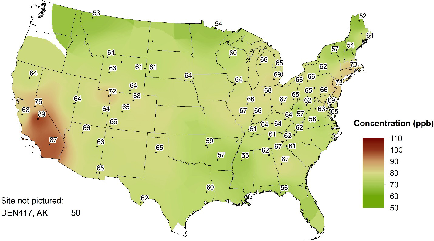
All CASTNET sites, with the exception of HOW191, ME; MCK231, KY; and ROM206, CO, are compliant under 40 CFR Part 58 and may be used for NAAQS compliance. HOW191 does not meet regulatory siting criteria. MCK231 and ROM206 are co-located sites used solely for QA purposes and are designated as “NAAQS excluded.” Three-year averages of the fourth highest DM8A O3 concentrations for 2015 through 2017 are presented in Figure 2-1. Ozone concentrations were not included on the map if the 3-year average was not available because of incomplete data; these sites are shown as dots with no value. Three California CASTNET sites, two eastern sites, and one site in Utah measured fourth highest DM8A O3 concentrations above the NAAQS of 0.070 ppm (EPA, 2015b). The highest 3-year design value of 89 ppb was sampled at the Sequoia and Kings Canyon National Parks, CA (SEK430) site. The highest 3-year eastern concentration (73 ppb) was measured at Washington Crossing, NJ (WSP144) and Abington, CT (ABT147). Table 2-1 lists sites with 2015–2017 O3 design values greater than 70 ppb.
An ozone design value describes the status of a given area with respect to the concentration values required by the ozone NAAQS. Design values change as each new 3-year period (e.g., 2015–2017, 2016–2018, etc.) of monitored ozone concentrations becomes available. Design values are used to classify nonattainment areas, develop control strategies to achieve the NAAQS, and to assess progress towards meeting the NAAQS. For an area to achieve the ozone NAAQS, the 3-year average of fourth highest DM8A ozone concentrations cannot exceed 0.070 ppm (EPA, 2015b). Designated criteria pollutant nonattainment areas are provided on the EPA website.
Figure 2-1 Three-year Averages of Fourth Highest DM8A O3 Concentrations for 2015–2017
 Download Figure
Table 2-1 Sites with Calculated Design Values for 2015–2017 greater than 70 ppb
| Site ID | State | Sponsor | 3-year Average |
|---|---|---|---|
| SEK430 | California | NPS | 89 |
| JOT403 | California | NPS | 87 |
| YOS404 | California | NPS | 75 |
| WSP144 | New Jersey | EPA | 73 |
| ABT147 | Connecticut | EPA | 73 |
| DIN431 | Utah | NPS | 72 |
Figure 2-2 shows 2017 fourth highest DM8A O3 concentrations that met percent completeness criteria. During 2017, three California sites, two eastern sites, and one site in Utah measured fourth highest DM8A O3 concentrations greater than 70 ppb. These are the same six sites with 2015–2017 design values greater than 70 ppb.
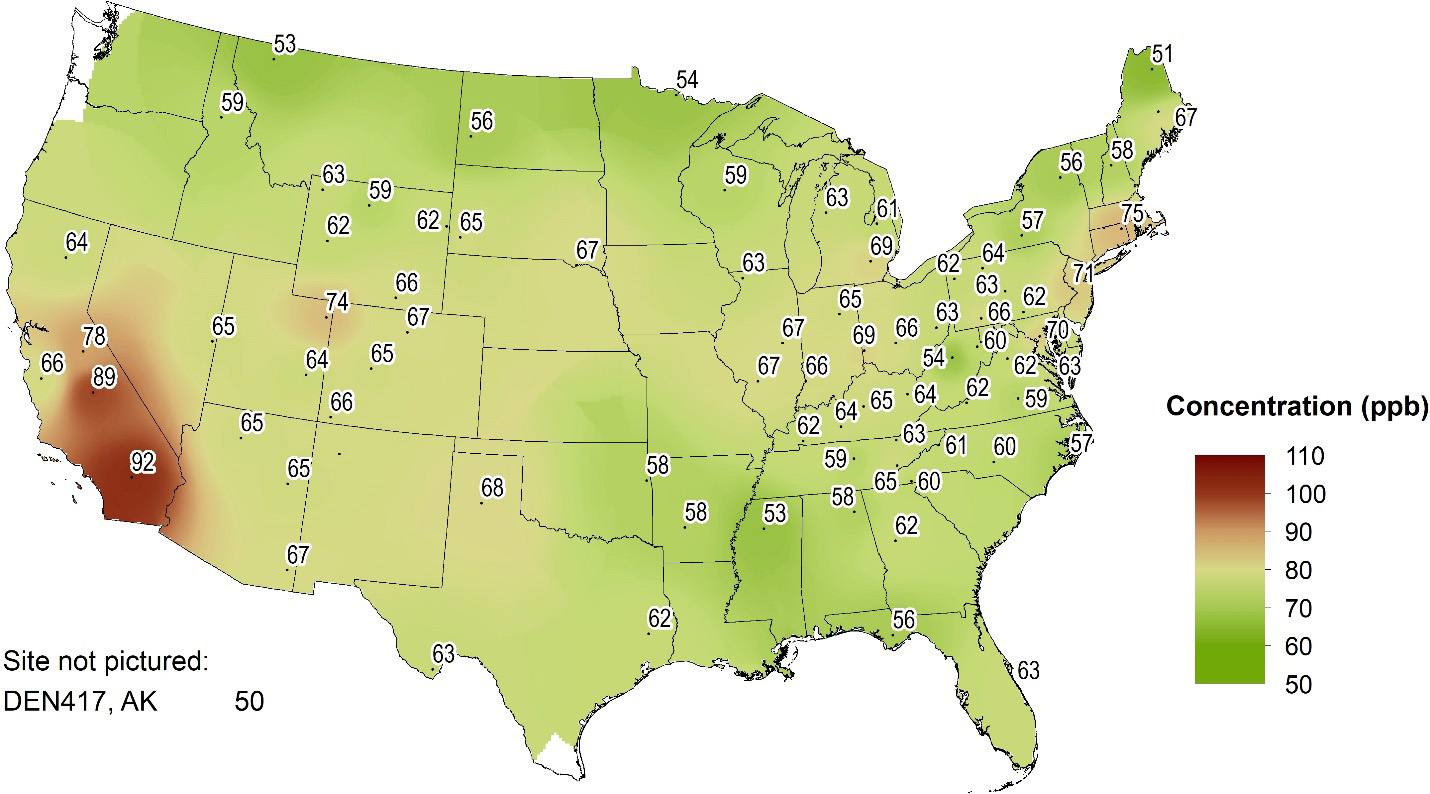
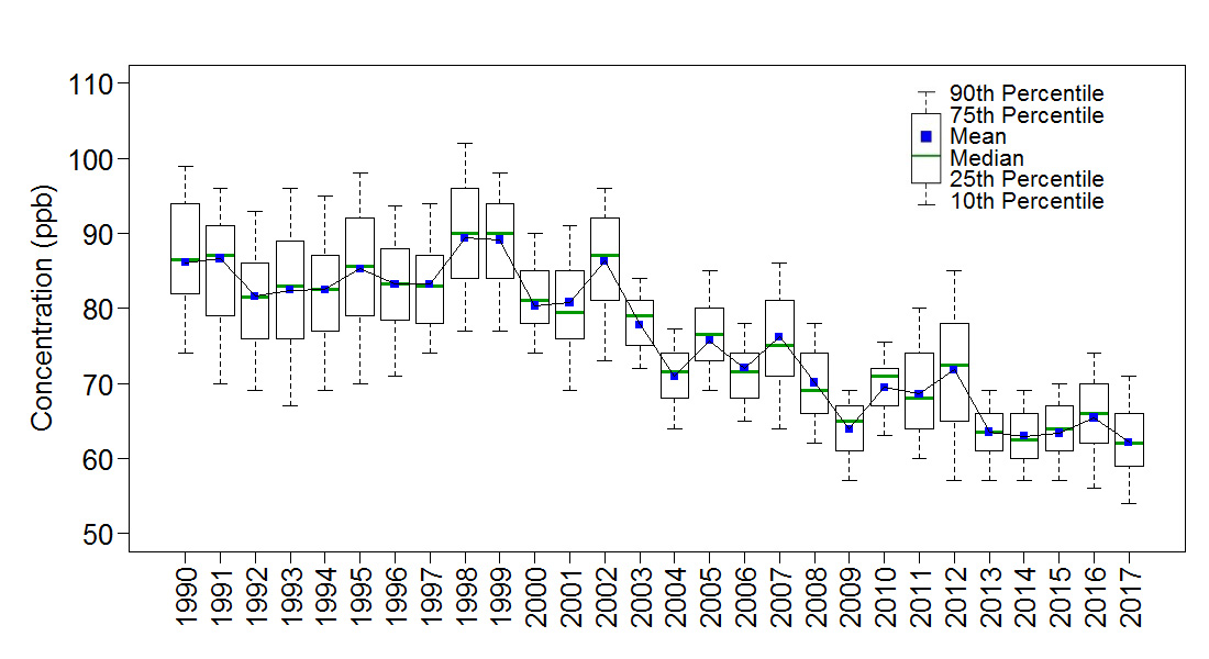
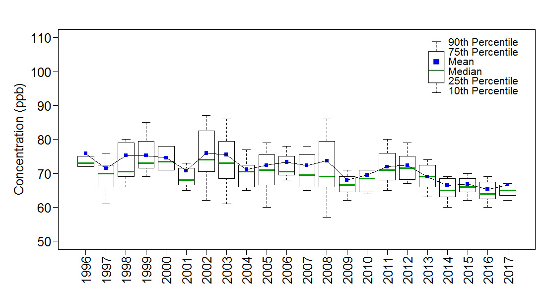
Figure 2-3 provides box plots depicting trends in 1-year mean, median, and annual distributions of fourth highest DM8A O3 concentrations from 34 eastern reference sites (top) for 1990 through 2017 and for 16 western reference sites (bottom) for 1996 through 2017. The reference sites were selected for their longterm data record and consistent performance. These sites were also used to show trends in ambient nitrogen and sulfur concentrations (Chapters 4 and 6).
The eastern O3 data show an overall decline of 24 percent in fourth highest DM8A O3 concentrations from 1990–1992 through 2015–2017. The 2017 median data point, 62 ppb, was the lowest in the history of the network.
The western O3 data show a reduction of 10 percent in fourth highest DM8A O3 concentrations from 1996–1998 through 2015–2017. The 2017 median of the fourth highest DM8A O3 concentrations for the western reference sites was 67 ppb, a slight increase from the 2016 concentration of 65 ppb.
Figure 2-3 Trends in Fourth Highest DM8A O3 Concentrations
Chapter 3: Stratospheric Ozone Intrusions
Certain weather conditions can transport ozone from the stratosphere to ground level at high-elevation sites primarily within the Intermountain Region of the western United States. These occasional intrusions of ozone-laden stratospheric air can contribute to atypically high ozone concentrations or even exceedances of ozone NAAQS. The EPA recently formed a workgroup of scientists and air quality managers from local, state, and federal agencies to provide support for identifying ozone stratospheric intrusions using a combination of model simulations, surface observations, and atmospheric sounding and satellite data. Examples of potential stratospheric ozone intrusions are discussed herein. The most prominent event occurred in Colorado and nearby states. Others happened at the Uintah and Ouray Reservation in the Uinta Basin, UT and in Thunder Basin, WY.
A stratospheric O3 intrusion occurs when O3-laden stratospheric air is transported across the tropopause and descends into the troposphere. Over the Intermountain West of the United States, intrusions may sporadically reach the ground at high elevations. They are rare at surface sites in the East due to the lower elevation. Stratospheric intrusions are identified by low tropopause heights, very low relative and specific humidity, low CO concentrations, and high concentrations of O3. Stratospheric intrusions that reach ground level typically occur in the spring and early summer, commonly follow strong cold fronts, and can extend across multiple states.
The identification of intrusions using only surface monitoring is difficult. Because intrusions are episodic, transient and localized, surface measurements along with vertical profile data from radiosondes, satellites, ozonesondes, and aircraft, if available, with supporting model simulations are needed to help demonstrate when intrusions contribute to high O3 concentrations at ground level. Satellite data show vertically integrated concentrations of O3, CO, and humidity. Low concentrations of CO and humidity, in conjunction with elevated O3 concentrations, give evidence of stratospheric air.
The EPA recently formed a workgroup of scientists and air quality managers from local, state, and federal agencies to provide support for identifying stratospheric intrusions. The group is called the EPA Ozone Stratospheric Intrusion Workgroup (SI Workgroup; Kaldunski et al., 2017). Examples of supporting analyses undertaken by the SI Workgroup to-date include:
- Analyses of O3 concentrations collected over surrounding regions;
- Descriptions of weather conditions, including an analysis of rapid spatial changes in 500 or 300 millibar (mb) flows, e.g., for sharp troughs;
- Presentation of Geostationary Operational Environmental Satellite System (GOES) satellite data including column-average O3, CO, relative humidity, and other parameters and their ratios;
- Estimates of tropopause height, isentropic potential vorticity (PV), and potential temperature;
- Presentation of upper air radiosonde data;
- Trajectory analyses, light detection and ranging, O3 profiles, satellite total column measurements, and atmospheric chemistry model simulations; and
- Regional model, e.g., Realtime Air Quality Modeling System (RAQMS) simulations (see the example in Figure 3-11).
The analyses included in this chapter are not intended to represent an exceptional events demonstration or to serve as examples of how to satisfy the Exceptional Events Rule criteria. For information about the Exceptional Events Rule and related guidance on stratospheric intrusion events, see https://www.epa.gov/air-quality-analysis/final-2016-exceptional-events-rule-supporting-guidancedocuments-updated-faqs.
Examples of Possible Stratospheric Ozone Intrusion – Colorado and Nearby States
The SI Workgroup identified a possible stratospheric intrusion event over parts of the Intermountain West on April 22–23, 2017. A detailed analysis of the April 2017 stratospheric intrusion event in Colorado and nearby states is presented first. The Ute Indian Tribe of the Uintah and Ouray Reservation documented high O3 concentrations influenced by stratospheric intrusion over the period June 8–15, 2015 in Uinta Basin, UT. The State of Wyoming Department of Environmental Quality/Air Quality Division (WDEQ/AQI) described a stratospheric intrusion event on June 6, 2012. These latter two examples are summarized at the end of the chapter.
Table 3-1 summarizes DM8A O3 concentrations measured over parts of the Intermountain West during the period of the suspected stratospheric intrusion on April 22, 2017. This table supplements the DM8A O3 concentrations displayed on the map in Figure 3-1.
Table 3-1 2017 DM8A O3 Concentrations
| Date | O3 (ppb) | Site* | State |
|---|---|---|---|
| April 22 | 82 | Gothic (GTH161) | Colorado |
| 80 | Navajo Lake | New Mexico | |
| 75 | Centennial (CNT169) | Wyoming | |
| 73 | Bloomfield | New Mexico | |
| 73 | Ute 1 | Colorado | |
| 72 | Coyote Ranger | New Mexico | |
| 72 | Mesa Verde National Park (MEV405) | Colorado | |
| 71 | Ute 3 | Colorado |
Note: *CASTNET site identification is included in parentheses. Ute 1 and Ute 3 ozone analyzers were operated by Southern Ute Indian Tribe in La Plata County, CO.
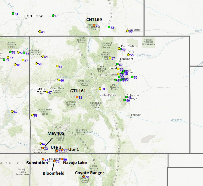
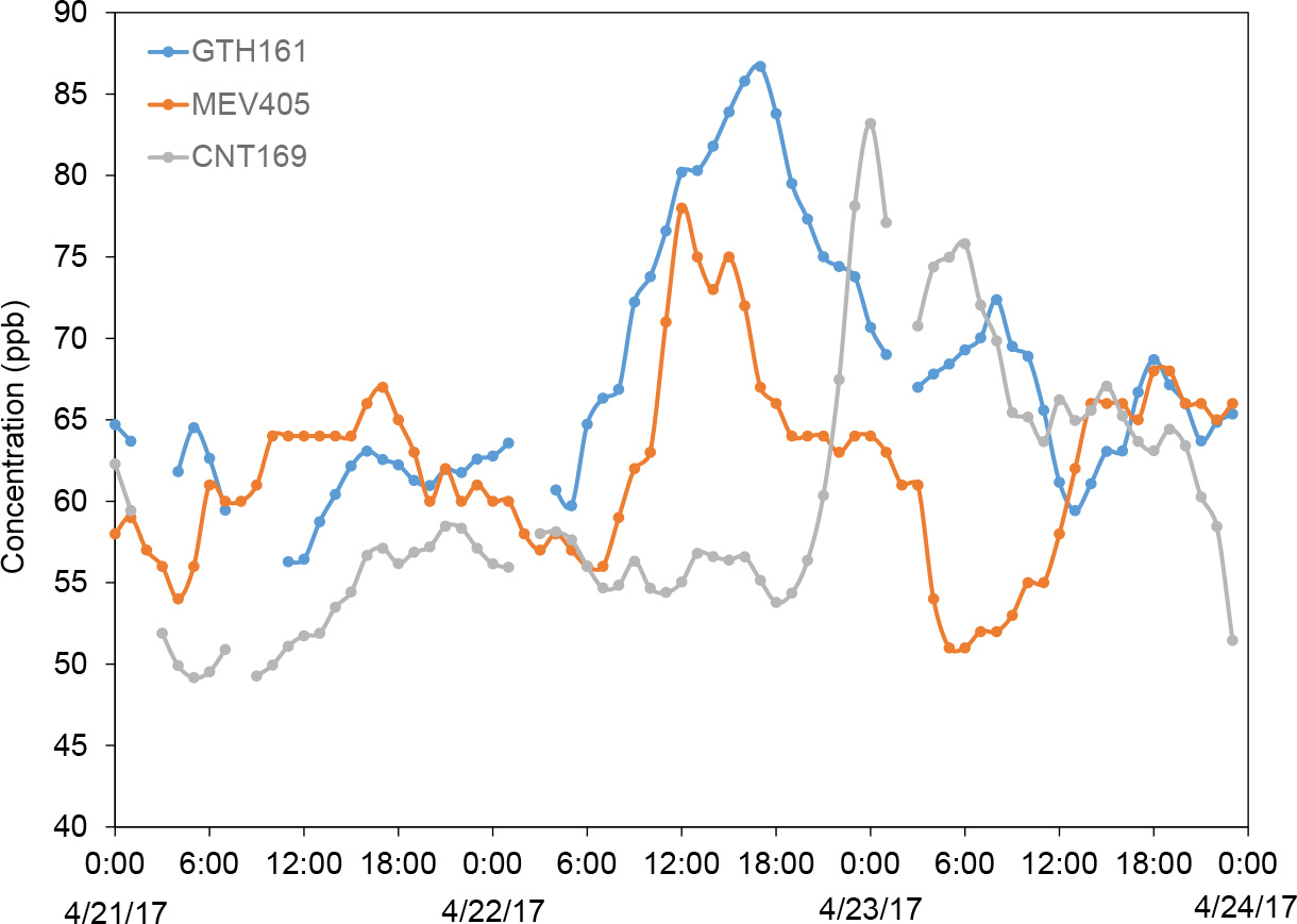
Figure 3-2 shows time series of hourly O3 concentrations measured at three CASTNET sites (GTH161, CNT169, and MEV405) over the period April 21–23, 2017. The time series show hourly O3 values at GTH161 exceeded 85 ppb on April 22, 2017.
Figure 3-2 Time Series of Hourly O3 Concentrations Measured at CASTNET Sites in Colorado and Wyoming
 Download Figure
The Colorado Department of Public Health and the Environment (CDPHE) requested that CASTNET managers append informational stratospheric intrusion flags (“IO”) to the hourly O3 values in EPA’s AQS to indicate to data users that these records may have been impacted by a stratospheric intrusion. The flagging request applies to GTH161 from April 22, 2017, 6:00 a.m. through April 23, 2017, 3:00 a.m. and to MEV405 from April 22, 2017, 9:00 a.m. through April 23, 2017, 7:00 a.m. (Harshfield, 2018).
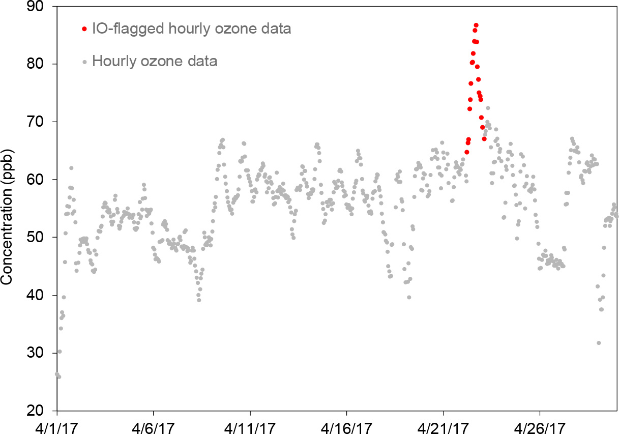
Figure 3-3 displays the abrupt increase and abrupt decrease of the IO-flagged O3 data at the time of arrival of the suspected stratospheric intrusion (orange). These records are shown with all valid hourly O3 data (gray) collected during the month of April 2017 from the GTH161 site. This month had a median hourly O3 concentration of 56 ppb and a median daily O3 production value of 11 ppb, i.e., the production of O3 from the minimum concentration typically around sunrise to the time of the maximum hourly concentration. This diurnal O3 profile is consistent with other Intermountain West sites.
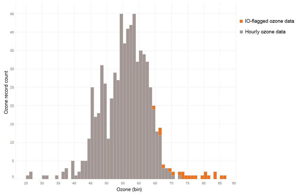
Figure 3-4 shows a histogram of valid hourly O3 records measured for the month of April 2017 with the April 22–23, 2017 IO-flagged hourly records highlighted in orange. The IO-flagged data were the highest values measured.
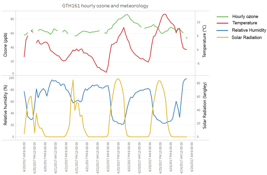
Hourly O3 and temperature measurements observed at GTH161 and supporting meteorological records from the Rocky Mountain Biological Laboratory’s Billy Barr weather station located approximately 1,000 m north-northwest of GTH161 are shown in Figure 3-5. The data were collected prior to the start of the suspected stratospheric intrusion to 48 hours after the end of the event. A negative correlation between solar radiation and relative humidity was recorded throughout the period. The drop in relative humidity on April 22, 2017, from 85 percent at 6:00 a.m. to 21 percent at 3:00 p.m., coincided with an increase in O3 concentrations from 64 ppb at 6:00 a.m. to 86 ppb at 3:00 p.m.
Figure 3-5 GTH161 Measured Hourly O3, Temperature, Relative Humidity, and Solar Radiation
 Download Figure
Source: https://www.digitalrmbl.org/collections/weather-stations/
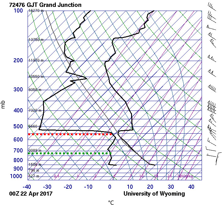
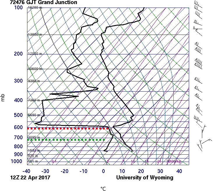
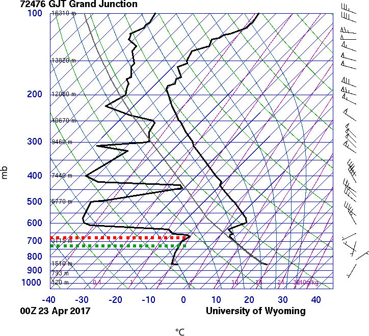
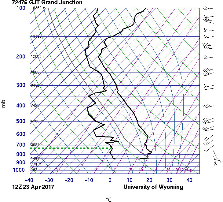
Additional information that helped identify the stratospheric intrusion was based on upper air sounding data from Grand Junction, CO, which is located approximately 85 miles west of GTH161. The data are plotted on Skew T log P diagrams (https://www.weather.gov/jetstream/skewt), which are commonly used to characterize vertical profiles of the atmosphere. In these plots, the bold black line on the left-hand side represents the sounding dew point and the bold black line on the right indicates the sounding temperature; the distance between these two lines is inversely proportional to relative humidity. The red dotted line that intersects the dew point line and extends to the y-axis identifies the lower bound altitude of a large dry air mass. The green dotted line shows the altitude (2915 m) of GTH161. The soundings were provided by the University of Wyoming.
The first three upper air sounding plots in Figure 3-6 illustrate the vertical descent of a parcel of dry air, which is demarked by a dew point temperature of -35 degrees Celsius (C). The parcel began at 550 mb at 5:00 p.m. on April 21 (Figure 3-6a), declined to 600 mb at 05:00 a.m. on April 22 (Figure 3-6b), and then to 650 mb at 5:00 p.m. on April 22 (Figure 3-6c), coinciding with the peak hourly O3 . The elevation of GTH161 is equivalent to a pressure level of about 720 mb. The fourth upper air sounding plot (Figure 3-6d) shows the dissipation of the presumed stratospheric air and the removal of the horizontal line that signified the dry air.
Table 3-2 summarizes the data in Figure 3-6 and illustrates how the lower bound altitude reached approximately 200-800 m above GTH161 while the temperature increased and relative humidity dropped during the elevated O3 event.
Table 3-2 Summary of Atmospheric Sounding Data April 21–22, 2017
| Pressure (mb) | Altitude (m) | O3 (ppb) | Temp (°C) | RH (%) |
|---|---|---|---|---|
| 550 | 5000-5600 | 62 | -1 | 82 |
| 600 | 4400-5000 | 60 | -8 | 86 |
| 675 | 3100-3800 | 87 | 4 | 49 |
| 720 | 2915 | 68 | -4 | 82 |
Note: RH = relative humidity
Figure 3-6 Upper Air Soundings Data for April 21, 2017, from 5:00 p.m. MST to April 23, 2017, 5:00 a.m. MST at Grand Junction, CO
Figure 3-6a. Upper air soundings data for April 21, 2017 at 5:00 p.m. MST (13 hours prior to the IO-flagged event).
 Download Figure
Figure 3-6b. Upper air soundings data for April 22, 2017 at 5:00 a.m. MST (one hour prior to the IO-flagged event).
 Download Figure
Figure 3-6c. Upper air soundings data for April 22, 2017, 5:00 p.m. MST coinciding with the peak hourly ozone.
 Download Figure
Figure 3-6d. Upper air soundings data for April 23, 2017 at 5:00 a.m. MST (two hours after the last IO-flagged data record).
 Download Figure
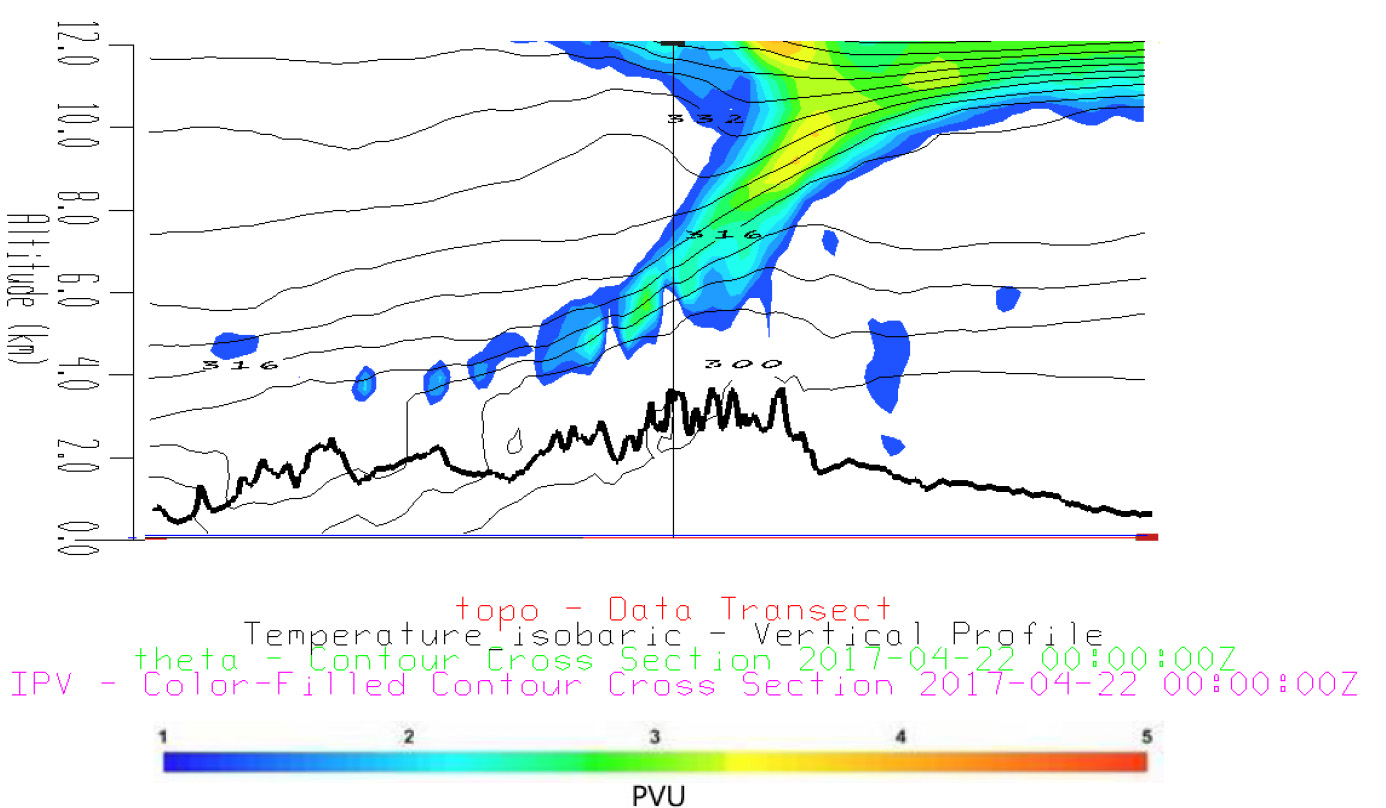
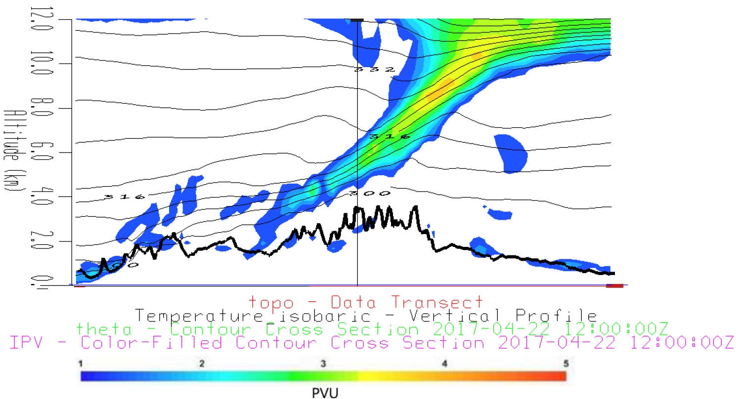
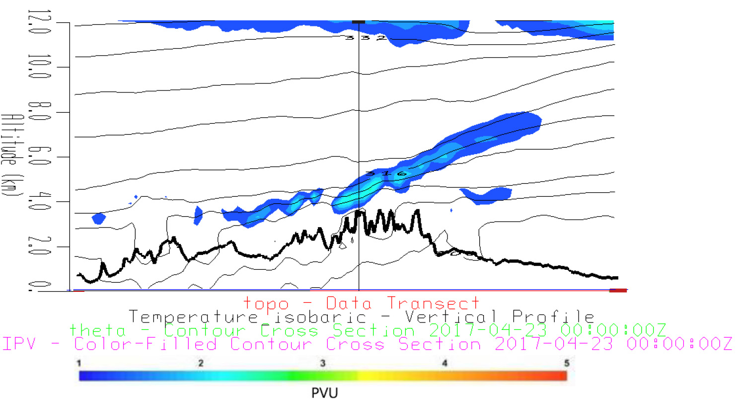
Figure 3-7 shows the North American Mesoscale (NAM) model vertical profiles of isentropic PV (color gradient), isobaric temperature (contour lines), ground surface topography (bold black line), and location of Gothic (black vertical line) for the period of April 21, 2017, 5:00 p.m. Mountain Standard Time (MST) through April 22, 2017, 5:00 p.m. MST at 12-hour increments. Potential vorticity was first identified as a tracer of stratospheric air in a study examining the exchange of stratospheric O3, radioactivity, and PV to the troposphere using aircraft and radiosonde measurement data (Danielsen, 1968). The plots in Figure 3-7 illustrate the sporadic nature of tropopause folds as measured by PV where exceedances of ~10-6 square meters per second (m 2/sec) times Kelvin/kilogram (K/kg) or one PV unit (PVU) 1 is a tracer for stratospheric air (Browell et al., 1987; Danielsen 1968; Danielsen et al., 1987; Xing et al., 2016).
The surface meteorological conditions and O3 concentrations shown in Figures 3-7a through 3-7c are the same as shown in Figure 3-6. A tropospheric fold appeared at approximately 1,000 to 2,000 m above the ground surface in Figure 3-7a. In Figure 3-7b the tropopause fold ranged from the ground surface to approximately 1,000 m above Gothic. The tropopause fold appears to touch the ground surface immediately above Gothic in Figure 3-7c.
1 PVU units are m 2/sec times K/kg.
Figure 3-7 NAM Meteorological Data for April 21, 2017 from 5:00 p.m. MST to April 22, 2017 5:00 p.m. MST Transect Across Gothic, CO
Figure 3-7a. NAM lateral transect for April 21, 2017 at 5:00 p.m. MST (13 hours prior to the IO-flagged event)
 Download Figure
Figure 3-7b. NAM vertical profile for April 22, 2017 at 5:00 a.m. MST (one hour prior to the IO-flagged event)
 Download Figure
Figure 3-7c. NAM vertical profile for April 22, 2017 at 5:00 p.m. MST coinciding with the peak hourly O3 concentration for the month of April 2017 of 87 ppb
 Download Figure
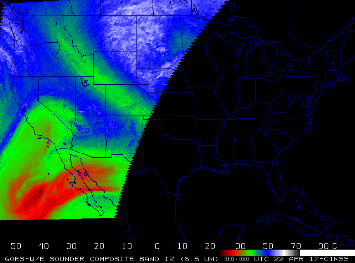
Figure 3-8 provides a GOES-derived satellite image of mid-level moisture measured on April 21, 2017 at 5:00 p.m. MST that shows a scattered band of air with low relative humidity (green) ranging from -30 to -40 °C from Idaho across Colorado.
Figure 3-8 GOES-Derived Satellite Images of Band 12 Mid-level Moisture on April 21, 2017 at 5:00 p.m. MST
 Download Figure
Figure 3-8 is approximately 13 hours prior to the start of the IO-flagged event.
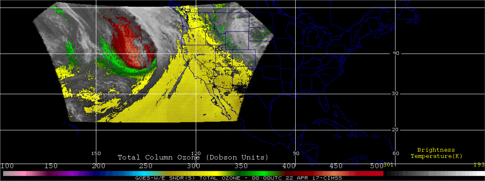
Figure 3-9 provides a GOES-derived satellite image of total column O3 measured on April 21, 2017 at 5:00 p.m. MST that shows a widely scattered band of O3 mixing ratios (green) ranging from 275 to 400 Dobson Units from Idaho across southwest Wyoming to southwest Colorado.
Figure 3-9 GOES-Derived Satellite Images of Total Column O3 on April 21, 2017 at 5:00 p.m. MST
 Download Figure
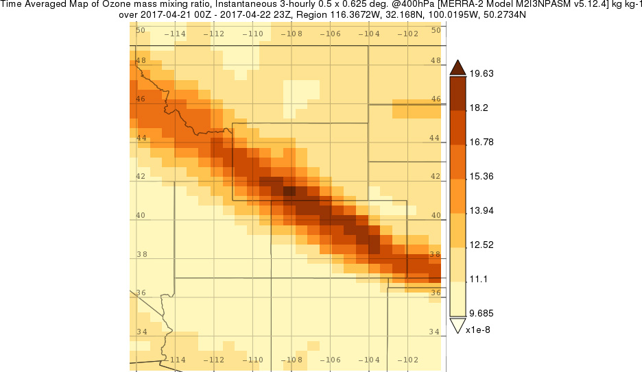
Figure 3-10 gives a Modern-Era Retrospective Analysis for Research and Applications, Version 2 (MERRA-2) image with a time-averaged O3 mass mixing ratio at 400 hectopascal (hPa 2; i.e., 400 mb) from April 21, 2017 from 5:00 p.m. MST (13 hours before the first IO-flagged data record) to April 22, 2017 at 4:00 p.m. MST (one hour before the peak hourly O3 measured at Gothic). This figure illustrates a distinct band of high O3 concentrations from the Idaho/Montana border across Colorado to the Oklahoma Panhandle.
Figure 3-10 MERRA-2 Average Ozone Concentrations at 400 hPa (mb) from April 21, 2017 5:00 p.m. MST to April 22, 2017 4:00 p.m. MST
 Download Figure
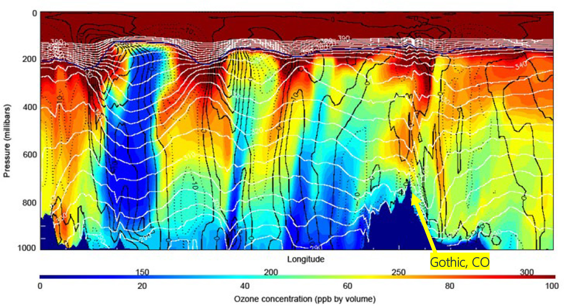
Figure 3-11 illustrates RAQMS simulations of the downward transport of O3 along a longitudinal crosssection at 40 degrees north (GTH161 is sited at 38.95627, -106.98587), which is located above the mountain peak silhouette (254.01 east longitude model location). The model results suggest a pocket of elevated O3 approached the ground surface near GTH161.
Figure 3-11 RAQMS Simulations of the Downward Transport of O3 along a Longitudinal Cross Section at 40 Degrees North
 Download Figure
In summary, the CDPHE requested that CASTNET managers append the IO informational stratospheric intrusion flags to the GTH161 and MEV405 hourly O3 values in AQS for April 22 and 23, 2017 to signify to data users that these records may have been impacted by a stratospheric O3 intrusion. Consequently, EPA, BLM, Wood scientists, and the SI Workgroup analyzed O3 data from GTH161, MEV405, and other sites; temperature and dew point soundings from Grand Junction; GOES satellite images; and various output from NAM and RAQMS model simulations to demonstrate that atypically high, ground-level O3 concentrations measured at GTH161 and MEV405 were likely influenced by a stratospheric intrusion.
Additional Examples of Stratospheric Ozone Intrusion – Ute Indian Tribe, Utah and Thunder Basin, Wyoming
Technical support for exceptional events documentation (Ute Indian Tribe of the Uintah and Ouray Reservation, 2016) was prepared for O3 NAAQS exceedances measured in the Uinta Basin, UT on June 8 and 9, 2015. EPA Region 8 scientists worked with the Tribe to analyze ozonesonde and satellite-based O3 data and RAQMS simulations. The Ute Indian Tribe operates O3 monitors at four locations in the Uinta Basin (Ouray, Redwash, Myton, and Whiterocks). CASTNET operates a monitor at Dinosaur National Monument (DIN431) in Utah. The four tribal monitors and DIN431 recorded their highest and second highest DM8A O3 concentrations in 2015 on June 8 and 9 (Table 3-3). Data presented in the exceptional events document show that high O3 concentrations measured on those days were unseasonably high, not consistent with historical readings and patterns, and coincided with the intrusion of stratospheric air into the troposphere contributing O3 to the surface measurements.
Table 3-3 Ute Indian Tribe of the Uintah and Ouray Reservation and DIN431 O3 Data during Period of Likely Stratospheric Intrusion (June 2015)
| Monitor Name | Monitor Number | 8-Jun-15 | 8-Jun-15 | 9-Jun-15 | 9-Jun-15 |
|---|---|---|---|---|---|
| DM8A O3 | Annual Rank | DM8A O3 | Annual Rank | ||
| Ouray | 49-047-2003 | 71 ppb | 1st | 71 ppb | 2nd |
| Redwash | 49-047-2002 | 74 ppb | 1st | 72 ppb | 2nd |
| Myton | 49-013-7011 | 71 ppb | 2nd | 72 ppb | 1st |
| Whiterocks | 49-047-7022 | 73 ppb | 1st | 73 ppb | 2nd |
| Dinosaur (DIN431) | 49-047-1002 | 74 ppb | 1st | 72 ppb | 2nd |
In another example of a stratospheric intrusion event, an exceptional event demonstration package was prepared for EPA for Thunder Basin, WY for an O3 NAAQS exceedance on June 6, 2012 by the WDEQ/AQD (2017). The Thunder Basin site is located in the northeast corner of the state. Table 3-4 shows the highest and second highest DM8A O3 concentrations in 2012 on June 6 and 7. During June 6, 2012, an upper atmospheric disturbance associated with a stratospheric intrusion moved over Wyoming likely contributing to elevated O3 readings resulting in a DM8A value of 88 ppb at the Thunder Basin O3 monitor. Additionally, the monitors at Gillette and Campbell County measured elevated 1-hour O3 values of 75 ppb during the stratospheric event. Concentrations also exceeded 70 ppb at South Pass and Boulder.
The WDEQ/AQD demonstration included statistical analyses of ground-level O3 measurements and an examination of hourly GOES total column O3 data, data from NASA’s Alpha Jet Atmospheric eXperiment (AJAX) Flight 47, and RAQMS and Rapid Refresh Model (RAP) simulations of O3, water vapor, and CO.
Table 3-4 Wyoming O3 Data During Period of Likely Stratospheric Intrusion
| Monitor Name | Monitor Number | 6-Jun-12 | 6-Jun-12 | 7-Jun-12 | 7-Jun-12 |
|---|---|---|---|---|---|
| DM8A O3 | Annual Rank | DM8A O3 | Annual Rank | ||
| Northeast Wyoming | |||||
| Thunder Basin | 56-005-0123 | 88 ppb | 1st | 52 ppb | 138th |
| Campbell County | 56-005-0456 | 75 ppb | 1st | 45 ppb | 158th |
| Gillette | 56-005-0800 | 75 ppb | 1st | 45 ppb | 162nd |
| West Wyoming | |||||
| South Pass | 56-013-0099 | 67 ppb | 4th | 73 ppb | 1st |
| Boulder | 56-035-0099 | 71 ppb | 3rd | 70 ppb | 4th |
| Daniel | 56-035-0100 | 67 ppb | 4th | 70 ppb | 2nd |
| Pinedale (WDEQ/AQD) | 56-035-0101 | 64 ppb | 7th | 69 ppb | 1st |
| Big Piney | 56-035-0700 | 68 ppb | 3rd | 69 ppb | 2nd |
The WDEQ/AQD concluded that a stratospheric intrusion event occurred during June 6, 2012 resulting in an exceptional event. Statistical analysis of June 6, 2012 data showed that the exceptional event was statistically significantly higher than data recorded during prior months of June from 2001 to 2012 at the Thunder Basin monitor. The stratospheric intrusion allowed O3-rich air to descend to the Thunder Basin monitor area and likely contributed to elevated 1-hour average O3 values.
Chapter 4: Nitrogen Pollutant Concentrations
During 2017, weekly average concentrations of nitric acid, particulate nitrate, and particulate ammonium were measured using 3-stage filter packs at 95 CASTNET monitoring stations. Maps of 2017 annual mean total nitrate (nitric acid plus nitrate) and ammonium concentrations illustrate the geographic distribution of the two pollutant indicators. Box plots show trends in annual mean total nitrate and ammonium concentrations aggregated over 34 eastern and 16 western reference sites. The nitrogen pollutants measured at the 34 eastern reference sites declined over the 28-year period from 1990 through 2017. At the eastern reference sites, annual mean concentrations of total nitrate were reduced by 51 percent, and ammonium concentrations declined by 68 percent. Total nitrate and ammonium concentrations measured at the 16 western reference sites were reduced by 37 percent and 32 percent, respectively, over the 22-year period 1996 through 2017.
Annual mean concentrations of total NO3- (HNO3 + NO3-) and NH4+ for 2017 are presented in two maps in this chapter. Trends in annual mean concentrations over the 28-year period, 1990 through 2017, were calculated from measurements from the 34 CASTNET eastern reference sites and for the 22-year period, 1996 through 2017, from data measured at the 16 CASTNET western reference sites. See Appendix A for the designated reference sites.
Trace-level gas analyzers measured NOy at six EPA and two NPS CASTNET sites during 2017. A new system for measuring all species of total reactive nitrogen, reduced plus oxidized, was added at the DUK008, NC site in May. Table 4-1 lists the site locations, start dates, and the trace-level gas parameters measured at the eight sites.
Table 4-1 Continuous, Trace-level Gas Monitoring Stations Operated at CASTNET Sites during 2017
| Site Location | Start Dates | Measurements |
|---|---|---|
| Mammoth Cave National Park, KY (MAC426)* | May 2009 | NO/NOy, SO2, and CO |
| Bondville, IL (BVL130) | July 2012 | NO/NOy, SO2, and CO |
| Huntington Wildlife Forest, NY (HWF187) | November 2012 | NO/NOy |
| Pinedale, WY (PND165) | May 2013 | NO/NOy |
| Cranberry, NC (PNF126) | October 2013 | NO/NOy |
| Rocky Mountain National Park, CO (ROM206) | October 2013 | NO/NOy |
| Great Smoky Mountains National Park (GRS420)* | November 2014 | NO/NOy, SO2, and CO |
| Duke Forest, NC (DUK008) | May 2017 | NO/NOy, SO2, and NHx |
Note: *Operated by NPS.
Total Nitrate Concentrations
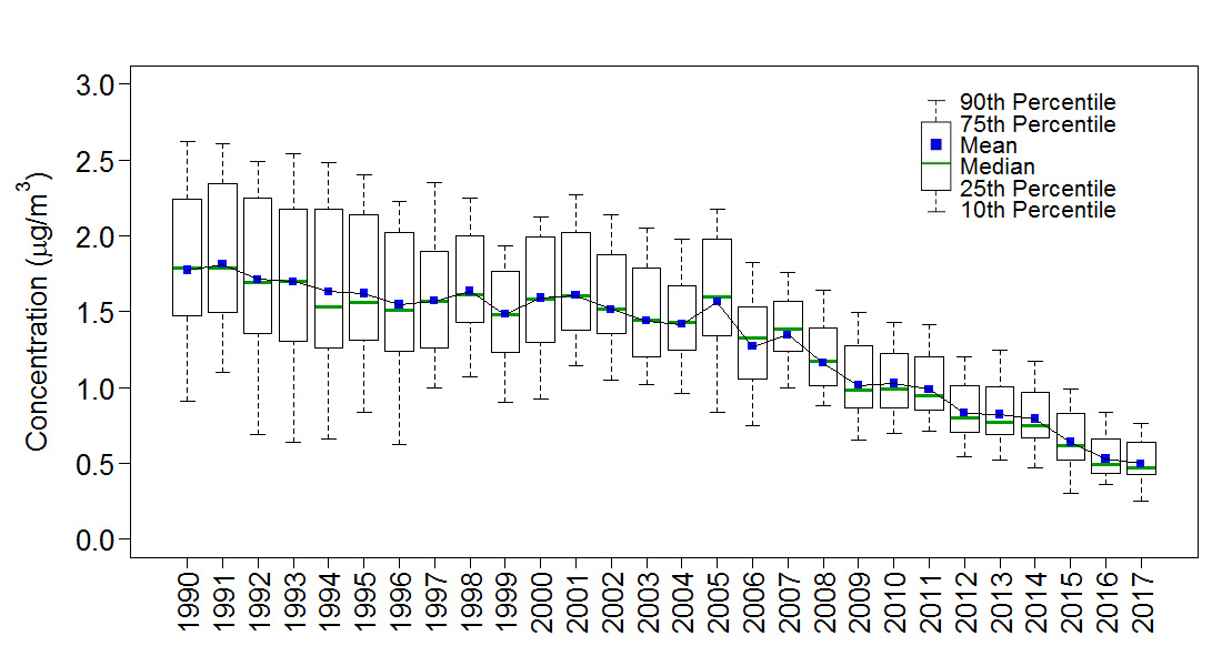
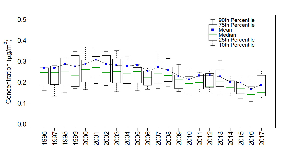
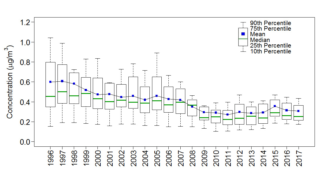
Mean total NO3- concentrations measured in 2017 are presented in the map in Figure 4-1. To illustrate trends, Figure 4-2 provides box plots of total NO3- levels for the eastern and western reference sites through 2017. Each box presents the mean and median concentrations and the 10th, 25th, 75th, and 90th percentiles for that year. The data shown in the upper half of the figure were aggregated from the 34 eastern reference sites. Over the history of the network, 3-year mean levels declined from 3.0 micrograms per cubic meter (µg/m 3) of air for 1990–1992 to 1.5 µg/m 3 for 2015–2017, producing a 51 percent reduction in total NO3-.
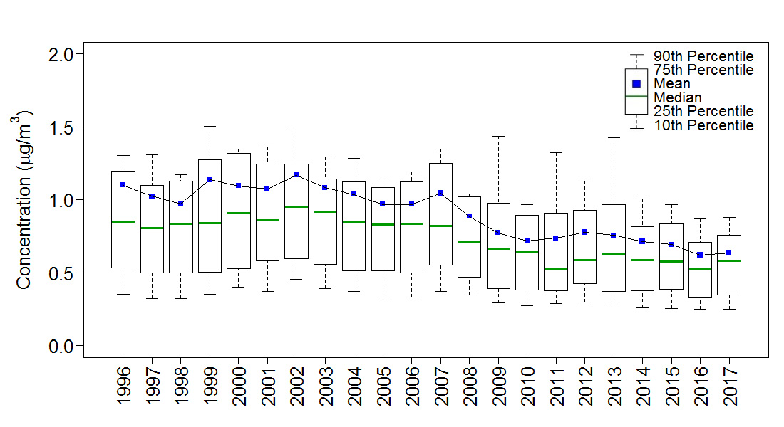
The lower half of Figure 4-2 shows data aggregated from the 16 western sites. The 3-year mean total NO3- concentration for 2015–2017 was 37 percent lower than the corresponding 1996–1998 level. The 3-year mean concentration was 1.0 µg/m 3 for 1996–1998 and 0.6 µg/m 3 for 2015–2017.
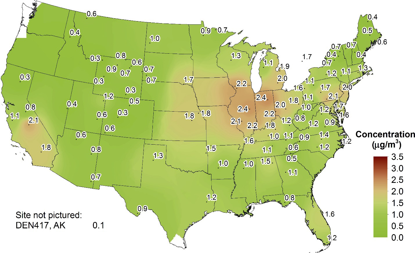
Figure 4-2 Trends in Annual Mean Total NO3- Concentrations
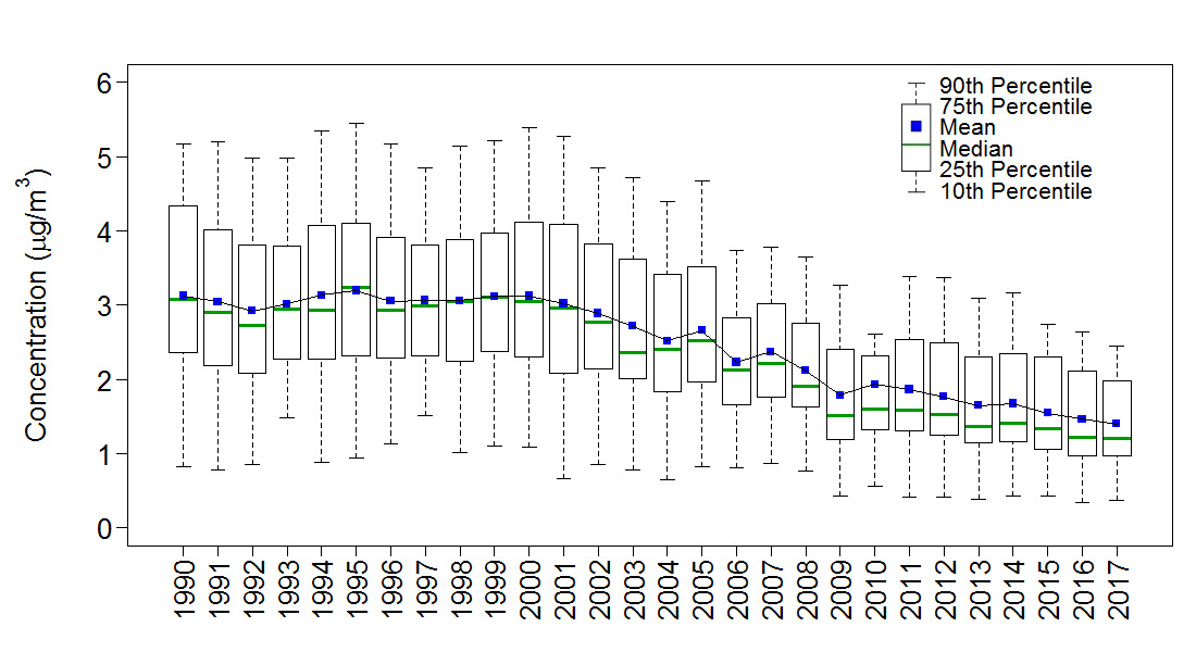
The 2017 average total nitrate concentration for the eastern reference sites was 1.4 µg/m 3 . The eastern total nitrate data show a substantive decline of 48 percent since 2000 with a reduction in 3-year mean total nitrate concentrations over the period 1990 through 2017 of 51 percent. This decline is less than the reduction (89 percent) in NOx emissions from EGUs operating in the eastern United States.
Particulate Ammonium Concentrations
A map of 2017 mean particulate NH4+ concentrations is provided in Figure 4-3. Figure 4-4 shows box plots of NH4+ concentrations. The trend diagram for the eastern sites (top) shows a reduction in mean NH4+ levels from 1990–1992 to 2015–2017. The 1990–1992 mean concentration was 1.8 µg/m 3 , and the 2015–2017 value was 0.6 µg/m 3 , a 68 percent decline. The western reference sites show a decline from 0.3 µg/m 3 in 1996–1998 to 0.2 µg/m 3 in 2015–2017, a 32 percent reduction.
Quality Assurance Program Results
Precision of Filter Pack Measurements
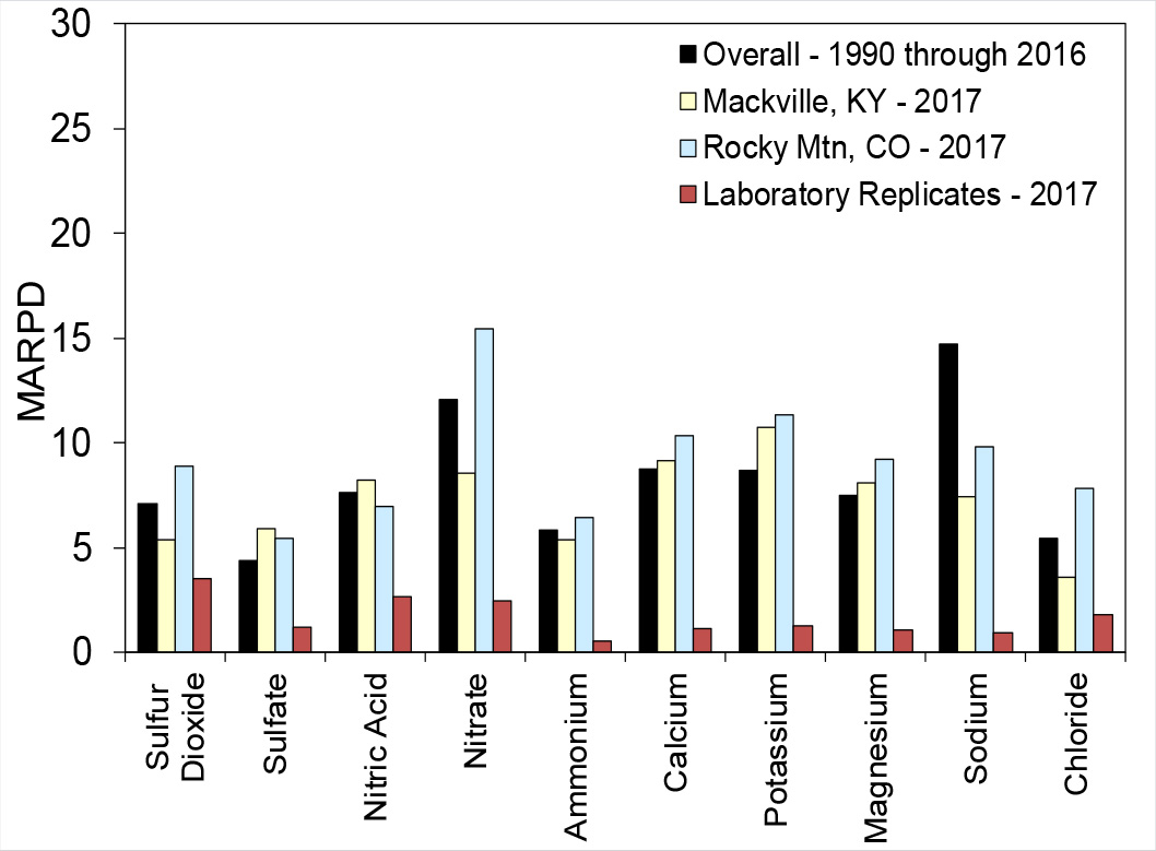
Historical (1990 through 2016) mean absolute relative percent difference (MARPD) data for all 11 co-located site pairs operated over the history of the network are provided in the bar chart in Figure 4-a. The 2017 data for the current co-located sites at MCK131/231 and ROM406/206 are also provided. The precision criterion is a MARPD of 20 percent. Historical and 2017 measurements met the criterion for each analyte.
Figure 4-a Historical and 2017 Precision Results for Atmospheric Concentrations and Laboratory Replicate Samples
 Download Figure
The 2017 analytical precision results for 10 analytes are also presented in Figure 4-a. The results were based on analysis of 5 percent of the samples that were randomly selected for replication in each batch. The results of in-run replicate analyses were compared with the original concentration results. The laboratory precision data met the 20 percent measurement criterion.
Data Completeness
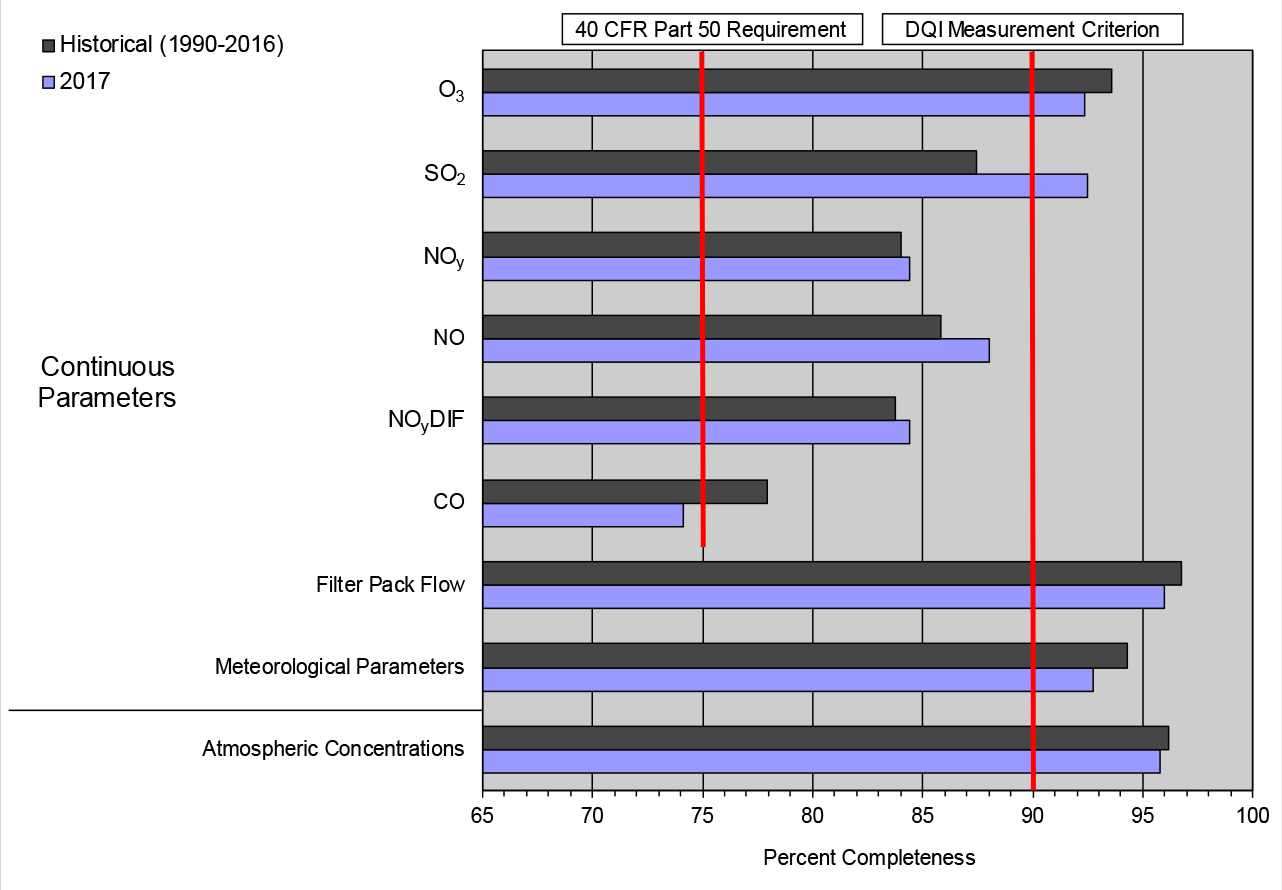
CASTNET measurements and supporting activities are assessed using DQI such as precision, accuracy, and completeness. Completeness is defined as the percentage of valid data points obtained from a measurement system relative to total possible data points. The CASTNET DQI measurement criterion for completeness requires a minimum completeness of 90 percent for every parameter for each quarter.
The historical results and the results for 2017 are given in Figure 4-b. Historical results for trace-level gas measurements represent data from 2013–2016. The completeness criterion was met for atmospheric (filter pack) and O3 concentrations, filter pack flow, and meteorological measurements. Completeness of trace-level gas measurements met the completeness requirements of 40 CFR Part 50 (EPA, 2015b) except for CO, which had a completeness less than 75 percent.
Figure 4-b Historical* and 2017 Percent Completeness of Measurements
 Download Figure
Note: *Black bars are 1990–2016 for long-term data and 2013–2016 for trace-level gas data
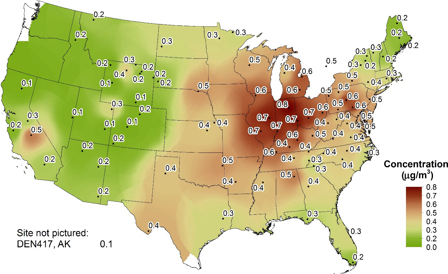
Figure 4-4 Trends in Annual Mean NH4+ Concentrations
Continuous Trace-level NOy and Filter Pack Total Nitrate Concentrations
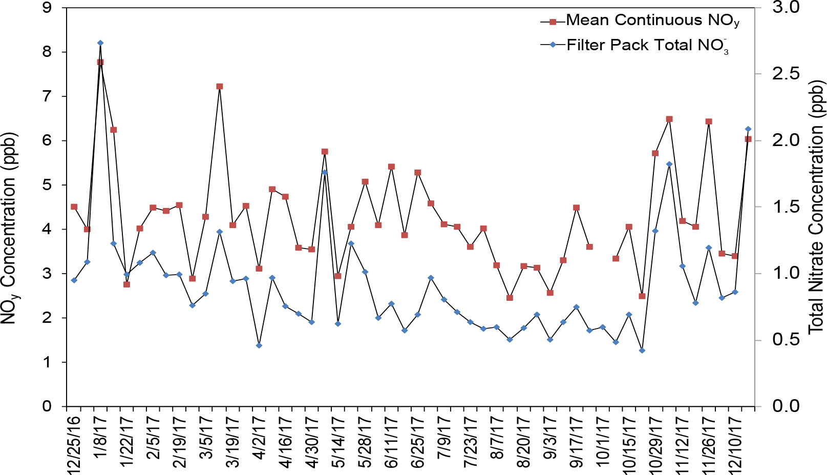
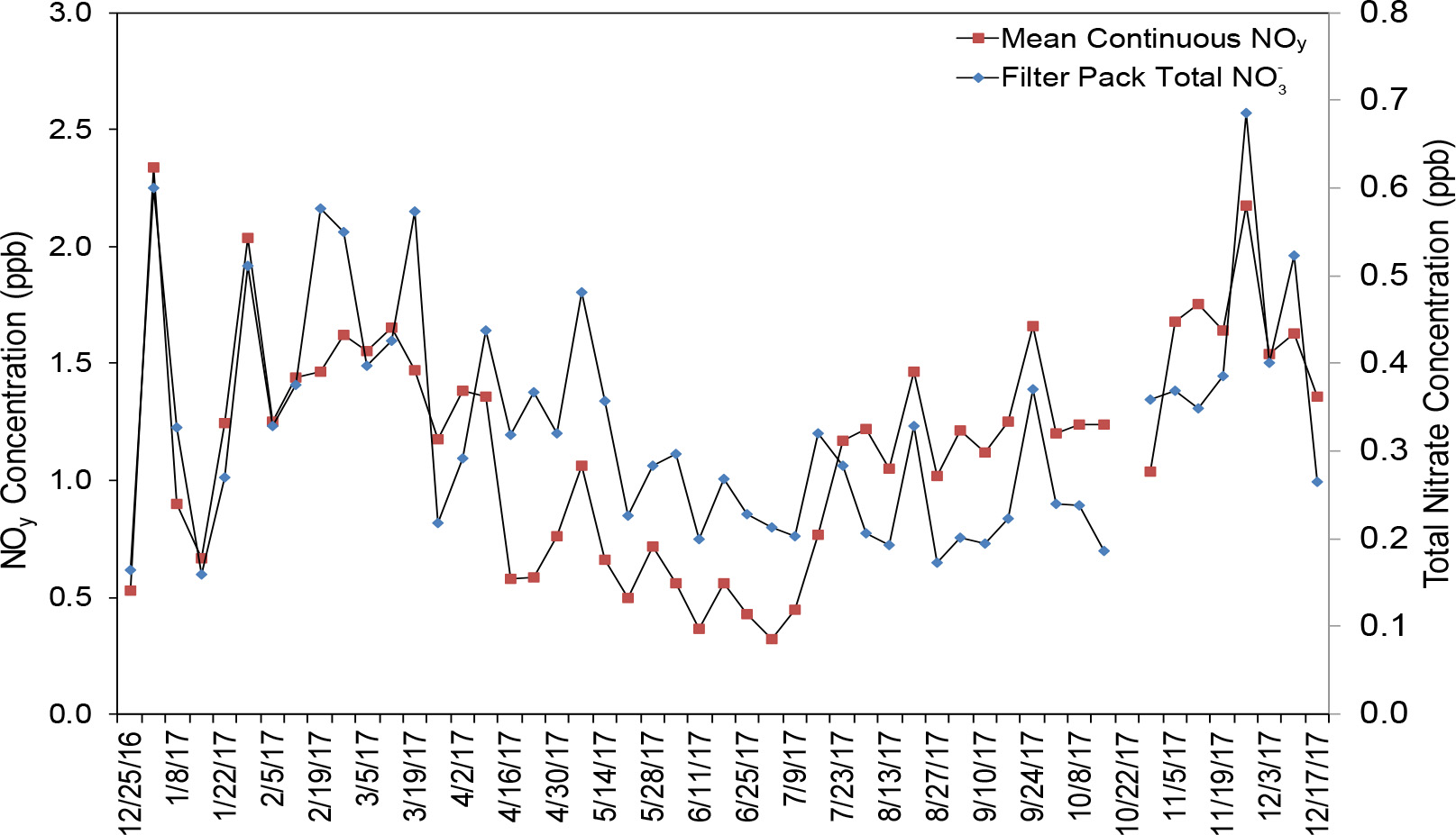
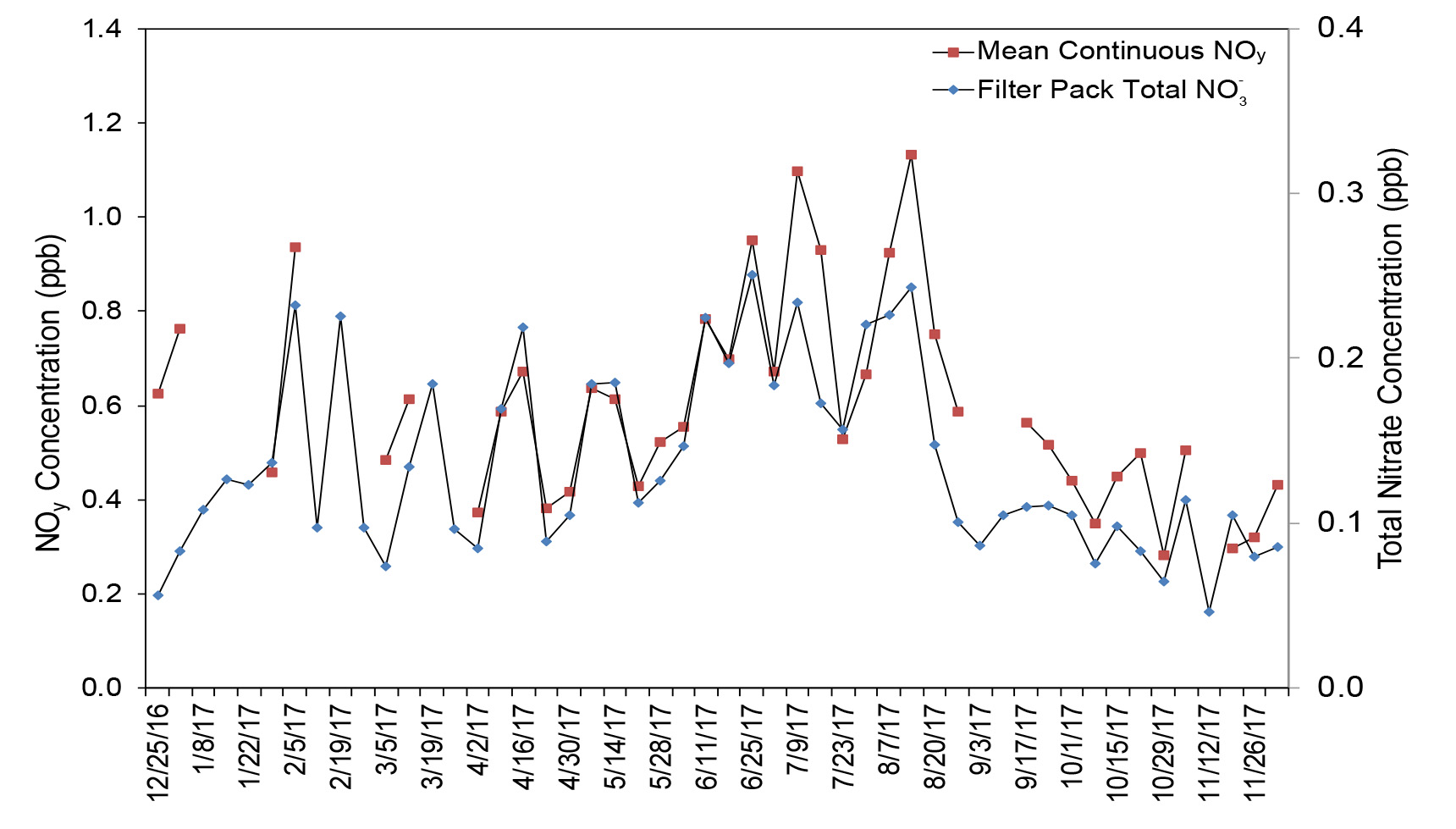
HNO3 and particulate NO3- are measured on CASTNET filter packs, and the sum is reported as total NO3-. NOy is defined as NOx (NO and nitrogen dioxide) plus NOz (HNO3, nitrous acid, peroxyacetyl nitrate, peroxyproyl nitrate, other organic nitrates, and nitrite). It consists of reactive gases that are considered precursors of O3 and PM2.5. Because HNO3 and particulate NO3- are measured as components of NOy, NOy concentrations should always be higher than total NO3- levels (i.e., the ratio of NOy to total NO3- should always be greater than 1.0). A comparison of weekly mean continuous NOy concentrations with filter pack total NO3- levels at BVL130, PNF126, and PND165 for 2017 was used to evaluate the measurements (Figures 4-5 through 4-7). The scales for NOy and total NO3- levels are different in the three figures. The NOy concentrations were consistently higher than the total NO3- levels, as expected. The results are similar for the other five sites. The weekly total NO3- concentrations, the average weekly NOy levels, and their ratios for all eight sites are listed in Table 4-2. These were calculated as the average of all valid weekly filter pack concentrations, the average of mean NOy values matching the run time of the weekly filter packs, and the average of the ratios calculated for each week. Weekly NOy levels were higher than the weekly total NO3- concentrations with ratios of NOy to total NO3- varying from 3.66 at PNF126 to 5.88 at ROM206.
Figure 4-5 Comparison of BVL130, IL Weekly Mean Continuous Trace-level NOy and Filter Pack Total NO3- Concentrations
 Download Figure
Figure 4-6 Comparison of PNF126, NC Weekly Mean Continuous Trace-level NOy and Filter Pack Total NO3- Concentrations
 Download Figure
Figure 4-7 Comparison of PND165, WY Weekly Mean Continuous Trace-level NOy and Filter Pack Total NO3- Concentrations
 Download Figure
Table 4-2 Summary of Total NO and NOy Measurements for 2017
| Site Location | Elevation (m) | Total NO (ppb) | NOy (ppb) | Ratio |
|---|---|---|---|---|
| DUK008, NC | 164 | 0.54 | 2.86 | 5.36 |
| BVL130, IL | 213 | 0.92 | 4.28 | 4.99 |
| MAC426, KY | 243 | 0.61 | 2.46 | 4.18 |
| HWF187, NY | 497 | 0.18 | 0.84 | 4.81 |
| GRS420, TN | 793 | 0.43 | 1.5 | 3.73 |
| PNF126, NC | 1216 | 0.33 | 1.16 | 3.66 |
| PND165, WY | 2386 | 0.14 | 0.6 | 4.54 |
| ROM206, CO | 2742 | 0.18 | 0.98 | 5.88 |
Chapter 5: Update on the Ammonia Monitoring Network
The Ammonia Monitoring Network (AMoN) operates passive ammonia samplers at 92 locations, 65 of which are located at CASTNET sites. AMoN is managed by the National Atmospheric Deposition Program. The network has been in operation since 2007 and provides information on 2-week integrated ammonia concentrations. The goal of AMoN is to operate a long-term (i.e., for several decades), spatially diverse network with consistent measurements across the continental United States.
Reduced nitrogen [ammonia (NH3) + NH4+] is an important component to total nitrogen deposition. Wet deposition of NH4+ measured by NTN has been increasing in many areas of the United States over the past 10 years; however, until 2007, gaseous NH3 concentrations were not routinely measured. Ammonia is the most prevalent alkaline gas in the atmosphere and is released into the air from a variety of agricultural sources (animal waste, fertilizer application, and agricultural burning), biological sources, gas and oil production and processing, and combustion. Agriculture is by far the largest source, producing approximately 80 percent of gaseous NH3 emissions (EPA National Emissions Inventory, 2014). Although NH3 is beneficial when used as NH3-based fertilizer, it can have a negative effect on the environment when it reacts with acidic ions such as SO42- and NO3- to form fine particulate matter (PM2.5), which contributes to negative impacts on human health and visibility degradation. Atmospheric deposition of reduced nitrogen also contributes to eutrophication of sensitive ecosystems, decreases in species diversity, and increases in invasive species.
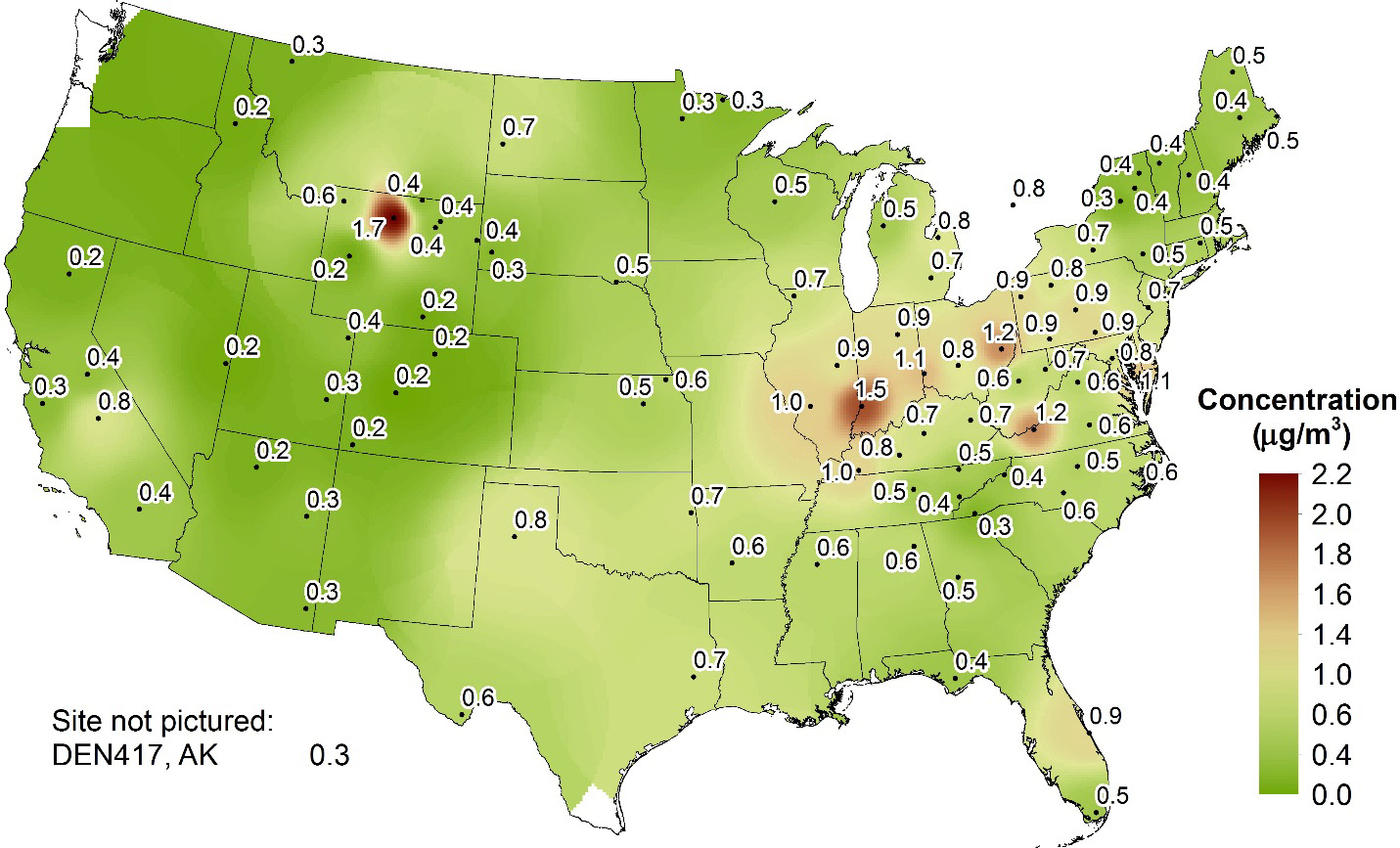
Average annual NH3 concentrations for 2017 for the sites that met completeness requirements are mapped in Figure 5-1 and show a wide range of concentrations from a low of 0.3 µg/m 3 at three sites in upstate New York (NY98), New Hampshire (NH02), and Nova Scotia (NS01) to a high of 16.9 µg/m 3 in northern Utah (UT01). The Utah monitoring site is located on a Utah State University research farm, and small quantities of livestock are often present (Martin and Baasandorj, 2016). The farm is situated in the Cache Valley, an area with frequently stagnant weather. The next highest concentrations ranged from 4.2 to 4.6 µg/m 3 at three sites west of the Mississippi River. The highest concentration east of the Mississippi was observed at Cranberry, NC (NC02) with a measured concentration of 5.2 µg/m 3 . High NH3 concentrations at this site can be attributed to local emissions from hog and cattle feeding and waste and crop fertilization and production.
Figure 5-2 provides box plots showing trends in NH3 concentrations from 2008 through 2017. The box plots were constructed with data from the 22 sites shown in Table 5-1. These sites were selected based on data completeness over the 10 years. The figure shows an increase in annual mean NH3 concentrations. In particular, 3-year mean concentrations increased from 1.32 µg/m 3 to 1.71 µg/m 3 (30 percent) from 2008-2010 through 2015-2017 and 3-year median concentrations increased by 16 percent from 1.11 µg/m 3 to 1.29 µg/m 3 . Two sites (TX43 and CO13) with relatively high concentrations reported the largest increases.
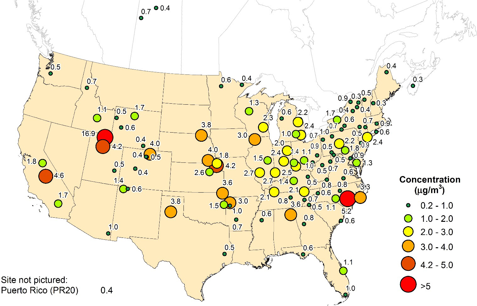
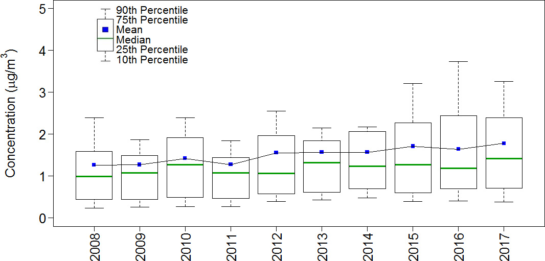
Table 5-1 AMoN Sites Included in Trends Analysis
| AMoN Site ID | Site Location/Name | State | CASTNET Site ID |
|---|---|---|---|
| CO13 | Fort Collins | CO | |
| ID03 | Craters of the Moon National Monument | ID | |
| IL11 | Bondville | IL | BVL130 |
| IN99 | Indianapolis | IN | |
| MD08 | Piney Reservoir | MD | |
| MD99 | Beltsville | MD | |
| MI96 | Detroit | MI | |
| MN18 | Fernberg | MN | |
| NC06 | Beaufort | NC | BFT142 |
| NC30 | Duke Forest | NC | DUK008 |
| NC35 | Clinton Crops Research Station | NC | |
| NM98 | Navajo Lake | NM | |
| NM99 | Farmington | NM | |
| NY16 | Cary Institute | NY | |
| NY67 | Ithaca | NY | CTH110 |
| OH02 | Athens Super Site | OH | |
| OH27 | Cincinnati | OH | |
| OK99 | Stilwell | OK | CHE185 |
| PA00 | Arendtsville | PA | ARE128 |
| SC05 | Cape Romain National Wildlife Refuge | SC | |
| TX43 | Cañónceta | TX | PAL190 |
| WI07 | Horicon Marsh | WI |
Chapter 6: Sulfur Pollutant Concentrations
Weekly average concentrations of sulfur dioxide and particulate sulfate were measured using 3-stage filter packs at 95 CASTNET monitoring stations during 2017. Maps of 2017 annual mean concentrations provide the geographic distribution of the two pollutants across the United States. Annual sulfur dioxide and sulfate concentrations were aggregated over 34 eastern and 16 western reference sites to show trends using box plots. The sulfur dioxide pollutants measured at the eastern reference sites declined by 89 percent over the 28-year period from 1990 through 2017. Particulate sulfate concentrations at the eastern reference sites were reduced by 75 percent. Sulfur dioxide and sulfate concentrations measured at the 16 western reference sites have decreased by 45 and 35 percent, respectively, over the 22-year period, 1996 through 2017.
Annual mean concentrations of SO2 and SO42- for 2017 are presented in this chapter. Trends in annual mean concentrations over the 28-year period, 1990 through 2017, were derived from measurements from the 34 CASTNET eastern reference sites and for the 22-year period, 1996 through 2017, from data measured at the 16 CASTNET western reference sites. See Appendix A for descriptions of the designated reference sites.
Sulfur Dioxide Concentrations
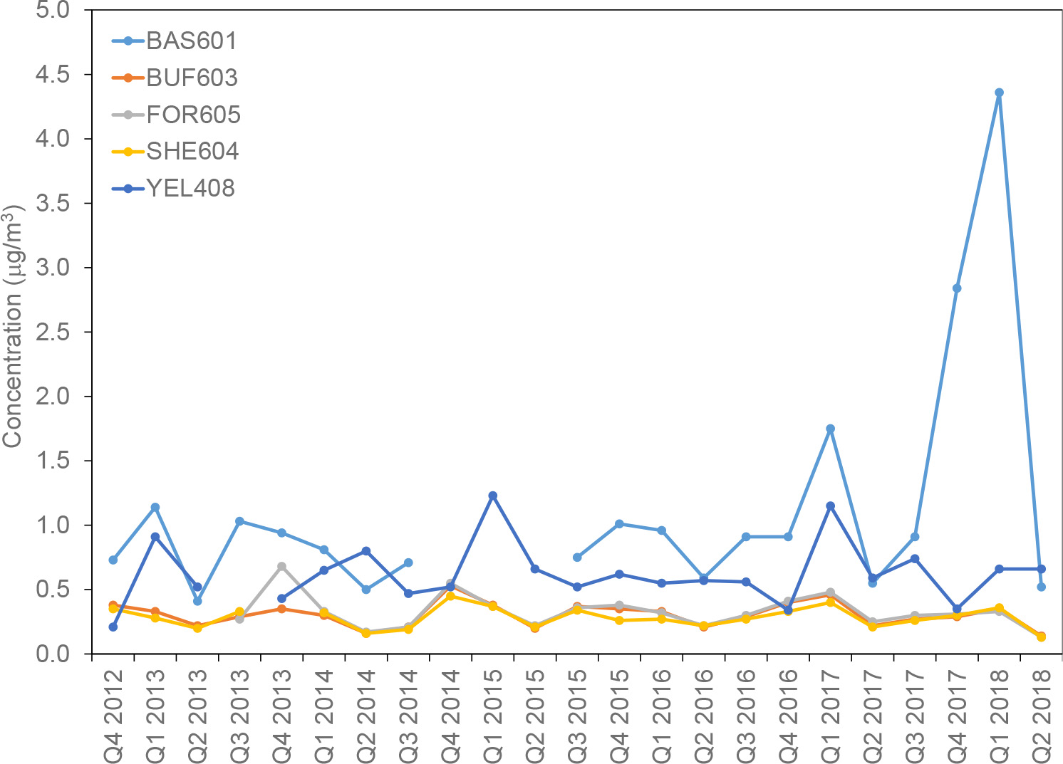
Annual mean SO2 concentrations for 2017 are shown in Figure 6-1. Annual mean concentrations were highest in the Midwest and East near and downwind of the Ohio River. The highest annual mean SO2 concentration was measured in the West at Basin, WY (BAS601), which measured unexpectedly high SO2 concentrations during fourth quarter 2017. See the additional discussion of BAS601 SO2 concentrations at the end of this chapter.
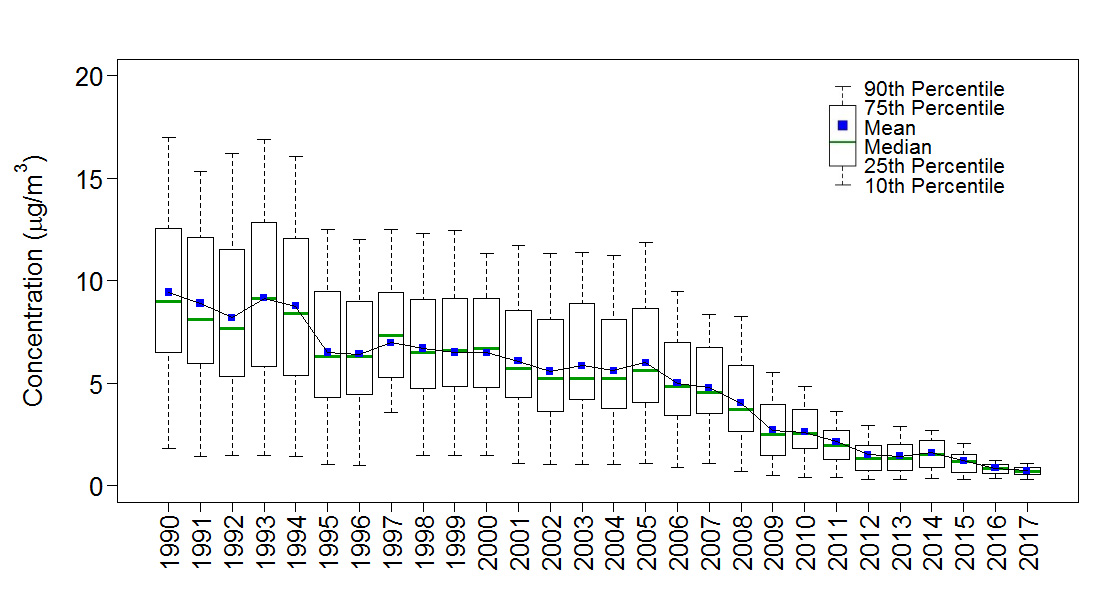
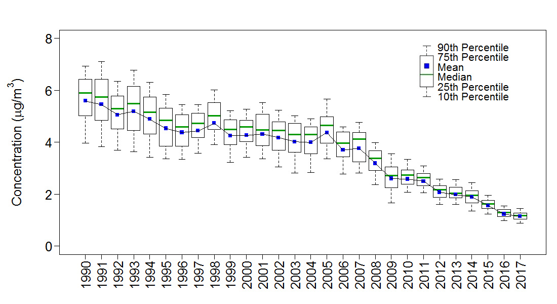
Box plots of annual mean SO2 concentrations aggregated over the 34 eastern reference sites from 1990 through 2017 (top) and the 16 western reference sites from 1996 through 2017 (bottom) are depicted in Figure 6-2. The y-axes on the western and eastern plots have different scales because concentrations measured at the western CASTNET sites were much lower than those measured at the eastern sites. Threeyear mean SO2 concentrations for the CASTNET eastern reference sites for 1990–1992 and 2015–2017 were 8.8 µg/m 3 and 0.9 µg/m 3 , respectively. This change constitutes an 89 percent reduction in 3-year mean SO2 concentrations between the two periods.
The box plots for the western reference sites indicate a decline in annual mean SO2 concentrations aggregated over the 16 sites. Three-year mean SO2 concentrations for 1996–1998 and 2015–2017 were 0.6 µg/m 3 and 0.3 µg/m 3 , respectively. This change constitutes a 45 percent reduction in 3-year mean SO2 concentrations at the CASTNET western reference sites over the 22 years.
The 2017 average sulfur dioxide concentration for the eastern reference sites was 0.7 µg/m 3 . The eastern sulfur dioxide data show a substantive decline since 1997. The reduction (89 percent) in sulfur dioxide concentrations over the period 1990 through 2017 is consistent with the reduction (96 percent) in sulfur dioxide emissions from EGUs operating in the eastern United States.
Figure 6-2 Trends in Annual Mean SO2 Concentrations
The trend in SO2 emissions from regulated EGUs from 1990 through 2017, aggregated over the eastern United States, was 96 percent, which is consistent with the 89 percent reduction (Figure 6-2) in annual mean SO2 concentrations aggregated over the CASTNET eastern reference sites.
Particulate Sulfate Concentrations
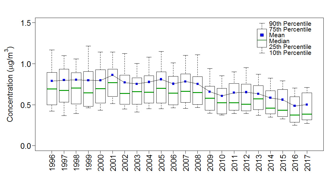
Figure 6-3 shows a map of 2017 annual mean particulate SO42- concentrations. Figure 6-4 provides box plots of annual mean SO42- concentrations from the 34 eastern reference sites and 16 western reference sites. The figure shows a substantial decline in SO42- over the 28 years for the eastern CASTNET reference sites. The difference between 3-year means from 1990–1992 to 2015–2017 depicts a 75 percent reduction in SO42- from 5.4 µg/m 3 to 1.3 µg/m 3 . The 2017 mean SO42- level of 1.1 µg/m 3 for the eastern reference sites was the lowest in the history of the network. The box plots for the western reference sites are provided on the lower half of Figure 6-4. The data show a 35 percent reduction in annual mean SO42- concentrations aggregated over the 16 sites with 1996–1998 and 2015–2017 concentrations of 0.8 µg/m 3 and 0.5 µg/m 3 , respectively.

The 2017 average sulfate concentration for the eastern reference sites was 1.1 µg/m 3 , the lowest level in the history of the network. The eastern sulfate data show a substantive decline since 2005. Sulfate concentrations declined more slowly than sulfur dioxide concentrations at the eastern reference sites. Western sulfate concentrations were lower and decreased at a slower rate than concentrations measured at the eastern sites.
Figure 6-4 Trends in Annual Mean SO42- Concentrations
Sulfur Dioxide Concentrations at Basin, WY
The BLM-sponsored site at Basin, WY (BAS601) is one of eight CASTNET monitoring sites in Wyoming (Figure 1-1). BAS601 measured unexpectedly high SO2 concentrations during fourth quarter 2017 causing concern about increased pollution. The data show the SO2 concentrations at BAS601 were consistently higher than levels measured at other Wyoming CASTNET sites (Figure 6-5). Although hundreds of oil and gas, mining, and other industrial facilities operate in the Bighorn Basin of Wyoming, no one particular activity can explain the high SO2 levels measured at BAS601. High concentrations persisted through first quarter 2018 and then returned to levels more consistent with the other Wyoming CASTNET sites.
Figure 6-5 Quarterly Mean SO2 Concentrations for Wyoming CASTNET Sites (Fourth Quarter 2012 through Second Quarter 2018)
 Download Figure
Chapter 7: Atmospheric Deposition of Nitrogen
CASTNET was designed to provide estimates of the dry deposition of nitrogen and sulfur pollutants across the United States. To assess the status of dry and total deposition for 2017, EPA used NADP’s Total Deposition Science Committee Hybrid Method. The hybrid method combines measured pollutant concentrations with output from the CMAQ modeling system. Total deposition was calculated as the sum of estimated dry and wet deposition.
Gaseous and particulate nitrogen pollutants are deposited to the environment through dry and wet atmospheric processes. A primary goal of CASTNET is to estimate the dry deposition of pollutants from the atmosphere to sensitive ecosystems. The NADP Total Deposition (TDep) Hybrid Method (EPA, 2015c; Schwede and Lear, 2014) combines CASTNET monitoring data with output from the CMAQ modeling system (Byun and Schere, 2006) to estimate dry deposition. The TDep method preferentially weights measurement data from air quality monitoring sites when available and to CMAQ output in areas where monitoring data are not available. In addition, CMAQ provides modeled data for species that are not routinely measured. The TDep method and its recent updates are discussed on the TDep web page. See also the NADP Fact Sheet, "Hybrid Approach to Mapping Total Deposition."
For wet deposition, the TDep method combines precipitation amounts measured at NADP/NTN sites with a PRISM-modeled grid of precipitation data. PRISM uses terrain elevation, slope, and aspect and climatic measurements to estimate precipitation. Pollutant concentrations in precipitation are measured by NADP/NTN, extrapolated into a grid using an inverse distance weighting algorithm, and then multiplied by the combined precipitation grid to generate a wet deposition surface. Dry and wet deposition fluxes were added to obtain estimates of total deposition, which are presented on the maps in this chapter as kilograms per hectare per year (kg ha -1 yr -1).
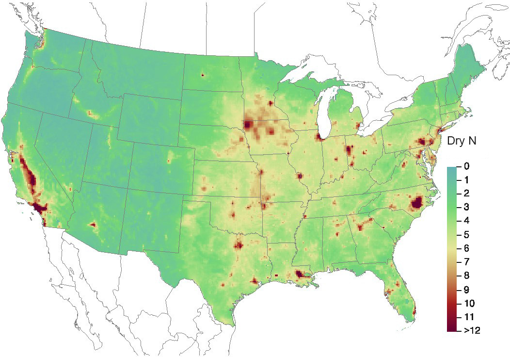
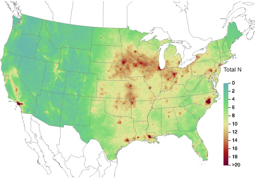
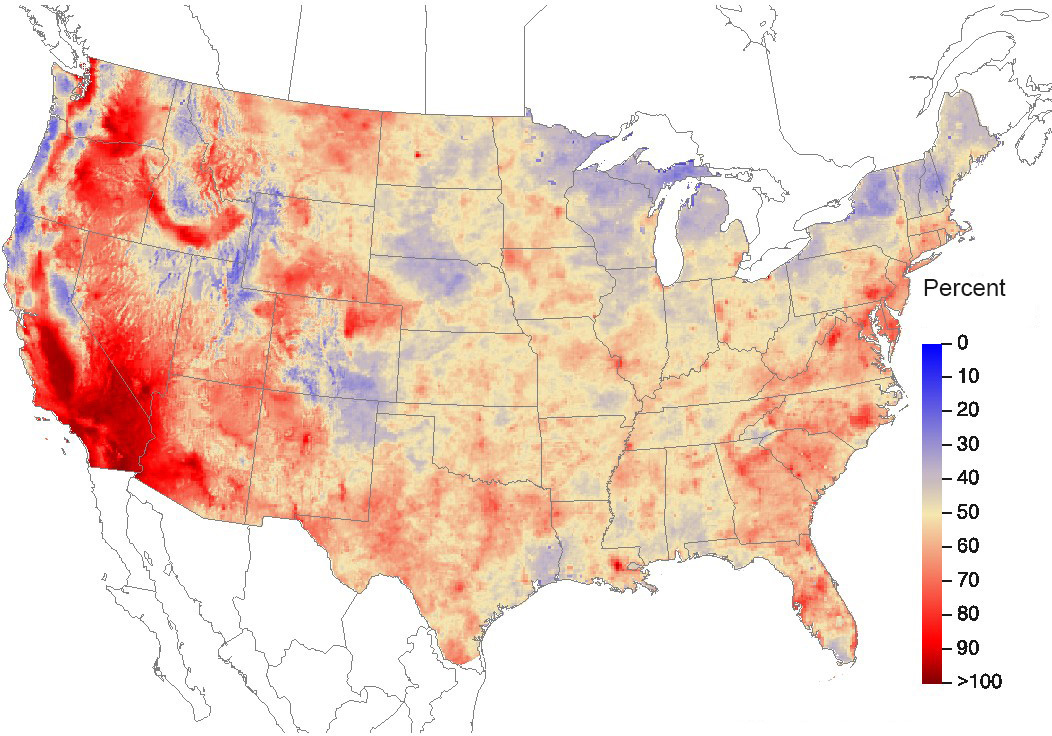
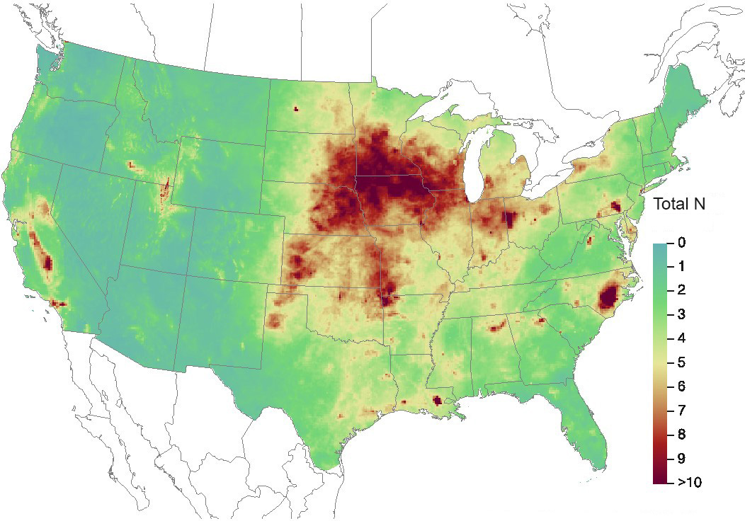
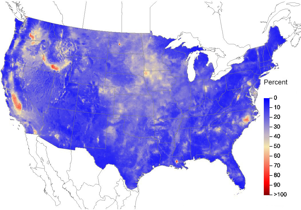
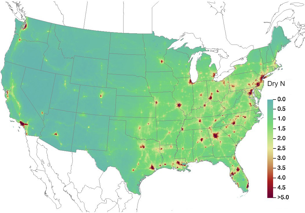
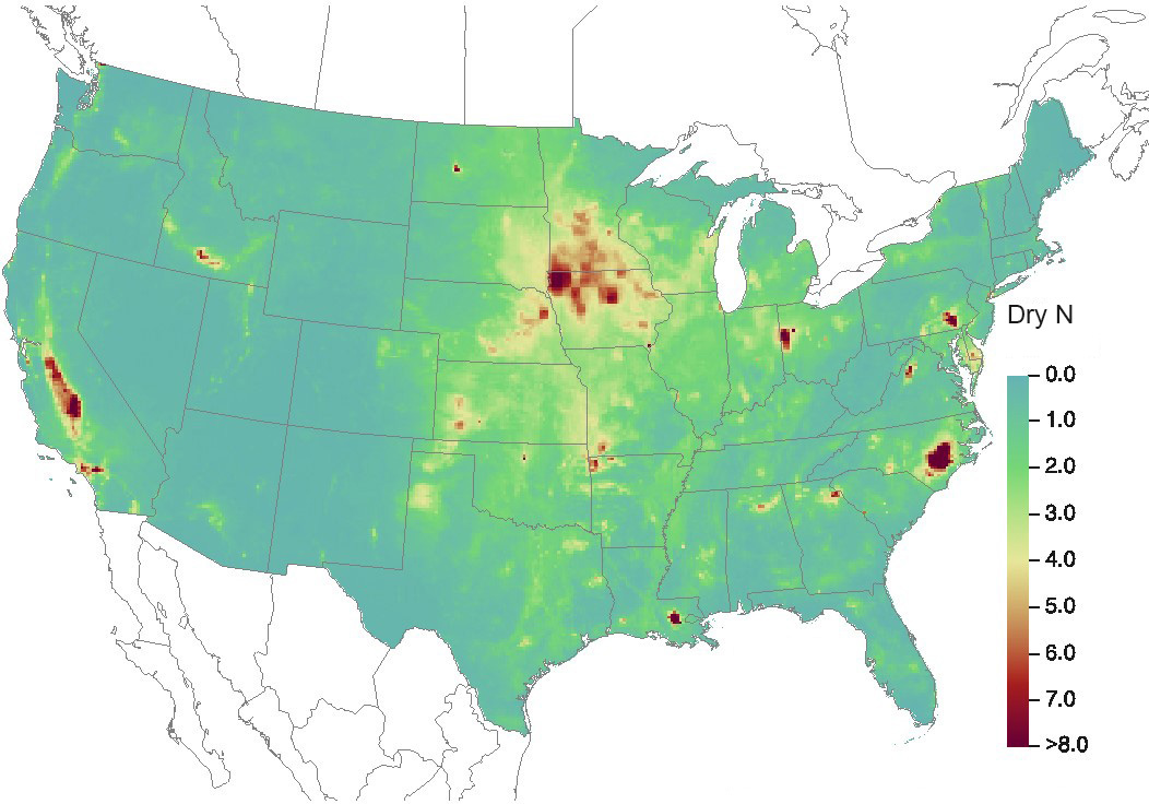
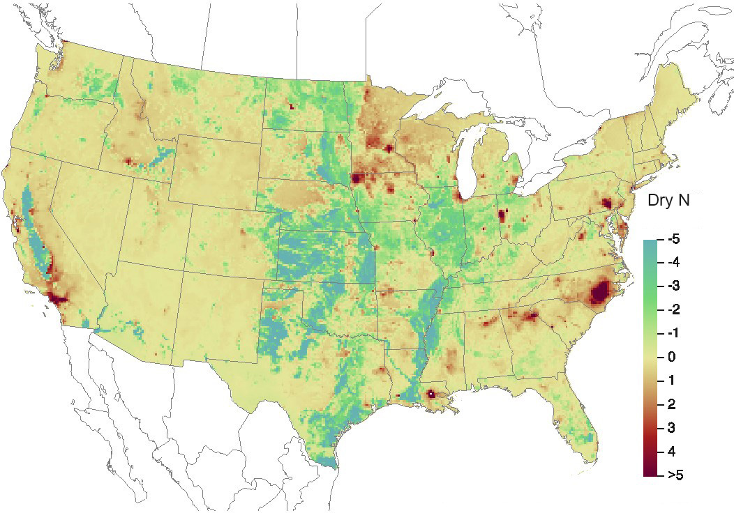
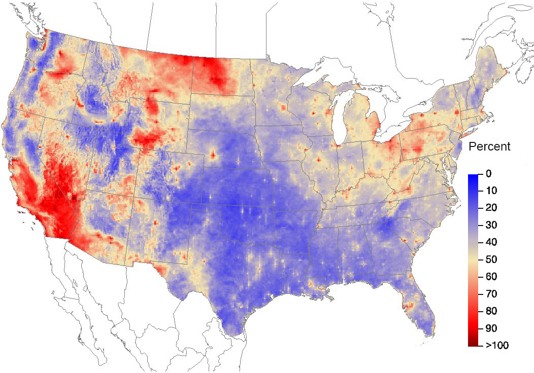
A map of the dry deposition fluxes of nitrogen (N) for 2017 generated by the TDep method is shown in Figure 7-1. The magnitude of the deposition fluxes is illustrated by the shading in the figure legend. A map of total deposition of N for 2017 is given in Figure 7-2. The percentage of total deposition of N due to dry deposition is shown in Figure 7-3. A map of TDep method estimates of total deposition of reduced N species for 2017 is given in Figure 7-4. Figure 7-5 gives the percentage of total deposition of reduced N species from dry deposition. Dry deposition of N species that are not routinely measured but are modeled by CMAQ and used in the TDep method is shown in the map in Figure 7-6, and its percentage of total deposition is shown in Figure 7-7. Annual gross dry deposition of NH3 for 2017 is shown in Figure 7-8, and the net dry deposition of NH3 is given in Figure 7-9. The net dry deposition figure shows the direction of the flux (i.e., positive values for deposition and negative values for emissions).
Figure 7-1 TDep Dry Deposition Estimates of N (kg ha -1 yr -1) for 2017
 Download Figure
Source: CASTNET|CMAQ|NADP
Figure 7-2 TDep Total Deposition Estimates of N (kg ha -1 yr -1) for 2017
 Download Figure
Source: CASTNET|CMAQ|NADP
Figure 7-3 TDep Percent of Total Deposition of N from Dry Deposition for 2017
 Download Figure
Source: CASTNET|CMAQ|NADP
Figure 7-4 TDep Total Deposition Estimates of Reduced N Species (kg ha -1 yr -1) for 2017
 Download Figure
Source: CASTNET|CMAQ|NADP
Figure 7-5 TDep Percent of Total Deposition of Reduced N Species from Dry Deposition for 2017
 Download Figure
Source: CASTNET|CMAQ|NADP
Figure 7-6 TDep Dry Deposition Estimates of Unmonitored N Species (kg ha -1 yr -1) for 2017
 Download Figure
Source: CASTNET|CMAQ|NADP
Figure 7-7 TDep Percent of Total Deposition of N from Dry Deposition of Unmonitored Species for 2017
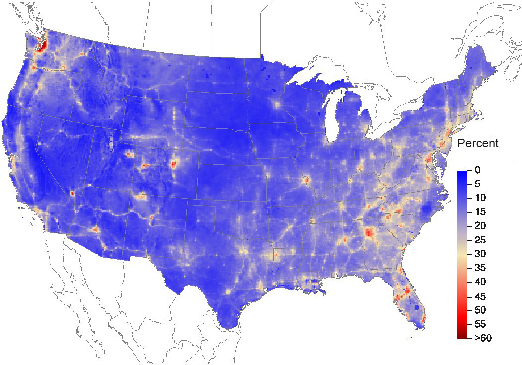 Download Figure
Source: CASTNET|CMAQ|NADP
Figure 7-8 TDep Gross Dry Deposition of NH3 as N (kg ha -1 yr -1) for 2017
 Download Figure
Source: CASTNET|CMAQ|NADP
Figure 7-9 TDep Net Dry Deposition of NH3 as N (kg ha -1 yr -1) for 2017
 Download Figure
Source: CASTNET|CMAQ|NADP
Chapter 8: Effects of California Wildfires on Air Quality
Wildfires and prescribed agricultural and forest management burns produce large amounts of aerosols and trace-level gases from burning vegetation, buildings, and other materials. Smoke from wildfires is a significant source of air pollution and can cause risks to health, visibility, and safety. The 2017 wildfire season was extensive with major fires in California in October and December. The October 2017 wildfires in Northern California were part of 250 wildfires that started burning across the state beginning in early October. These wildfires affected Napa, Sonoma, Lake, Mendocino, Butte, and Solano counties. Twentynine wildfires ignited across Southern California in December 2017. The Thomas Fire, which started on December 4, affected Ventura and Santa Barbara counties. CASTNET ozone measurements and air quality data from local air pollution control districts showed elevated levels of ozone and fine particulate matter during the California wildfire events.
Wildfire smoke is a mixture of CO, volatile organic compounds, PM2.5, and smaller particles that include alkaline ash, black and organic carbon, and polyaromatic hydrocarbons. Wildfire smoke is also a precursor to downwind O3 concentrations. The 2017 wildfire season was extensive with major fires in California in October and December. Wildfires were not confined to the West. In late November, major fires were reported in Arkansas, Kansas, Kentucky, Missouri, Oklahoma, and Pennsylvania (Peltier, 2017). Measurements from CASTNET and other federal, state, and county networks provided information to characterize the impacts of wildfires on air quality and visibility near critical resources. Measurements from local air pollution control districts (APCDs) and AirNow (https://www.airnow.gov/) provided additional information.
Northern California Wildfires
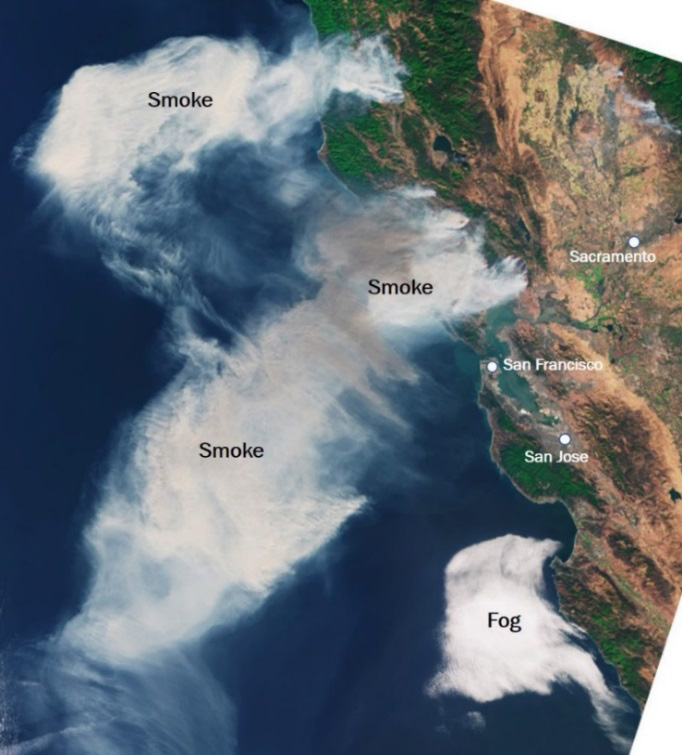
The October 2017 Northern California wildfires were part of 250 wildfires that started burning across the state beginning in early October. Twenty-one became major fires that burned at least 245,000 acres. Fires started on the evening of Sunday, October 8, with the largest fires occurring in Napa and Sonoma counties. Weather and dry vegetation at the time were favorable for rapid fire growth. The wildfires spread throughout Napa, Sonoma, Lake, Mendocino, Butte, and Solano counties during severe fire weather conditions (CAL FIRE, October 30, 2017).
Figure 8-1 shows satellite images (Alrick, 2018) of the smoke plumes from the fires in Northern California. A daily weather map for October 9, 2017 [National Oceanic and Atmospheric Administration (NOAA), 2017] is given in Figure 8-2. A strong pressure gradient between the Bay Area and a surface high over Idaho resulted in brisk offshore winds that spread the fires.
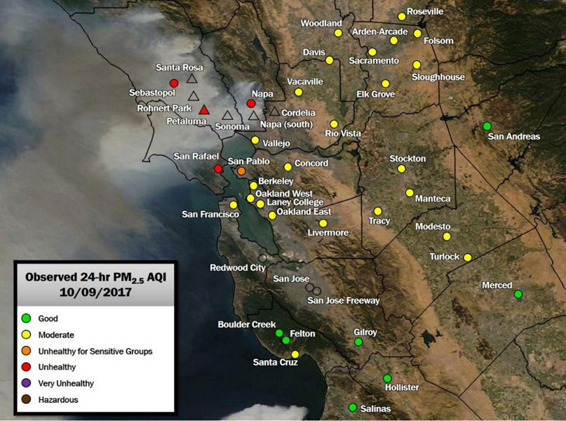
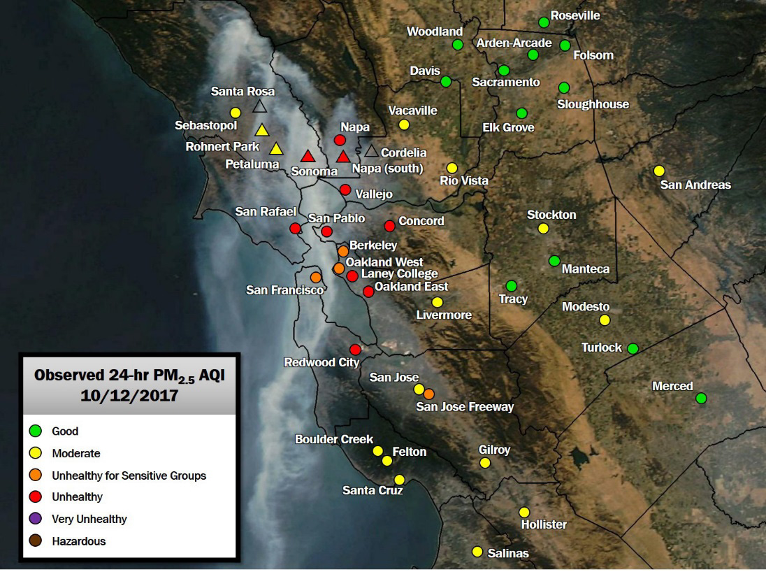
An air quality index (AQI) is a form of measurement used by EPA and other governmental agencies to inform the public about levels of air pollution in their communities. Figure 8-3 provides a map of daily average PM2.5 concentrations color-coded by the AQI category for each area on October 9.
Figure 8-1 Satellite Image of October 2017 Northern California Wildfires
 Download Figure
Source: Alrick, 2018
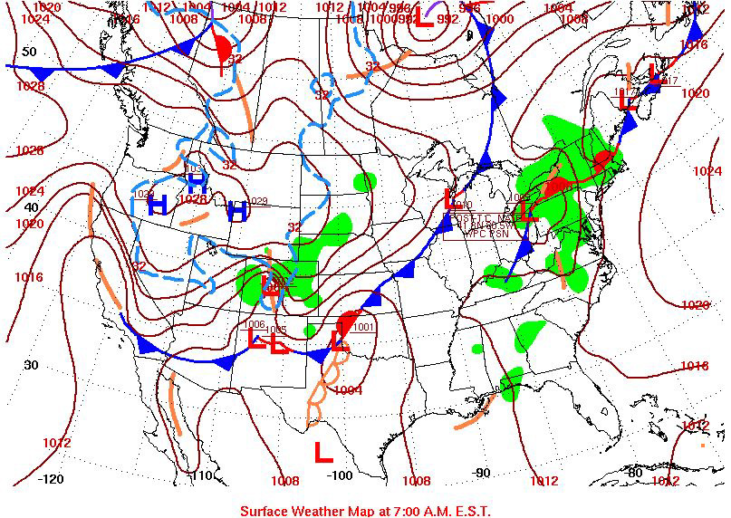
Figure 8-3 Map of Daily Average PM2.5 Concentrations (µg/m 3 ) Color-Coded by AQI Category for October 9, 2017
 Download Figure
Source: Alrick, 2018
The winds switched to more northerly by October 12 and varied throughout the period October 8 through October 19. By October 12 (Figure 8-4), smoke from the wildfires had spread nearly 100 miles, registering "unhealthy" AQI in the cities of Oakland, San Francisco, and San Rafael. Downwind from the fire, the air quality in the city of Napa was ranked the poorest in the nation due to high levels of PM2.5 and O3 (Ho and Lyons, 2017).
Figure 8-4 Map of Daily Average PM2.5 Concentrations (µg/m 3 ) Color-Coded by AQI Category for October 12, 2017
 Download Figure
Source: Alrick, 2018
Southern California Wildfires
Twenty-nine wildfires ignited across Southern California in December 2017. Six of the fires became significant wildfires that led to widespread evacuations and property losses. The wildfires burned over 307,900 acres and caused high air pollutant concentrations, traffic disruptions, school closures, and power outages. The largest of the wildfires was the Thomas Fire, which grew to 281,893 acres. These wildfires were exacerbated by unusually powerful and long-lasting Santa Ana winds and large amounts of dry vegetation, due to an extensive dry period following the 2016–2017 rainy season. The Santa Ana winds also occurred at the end of an active and destructive wildfire season in 2016 (Byrne, 2018).
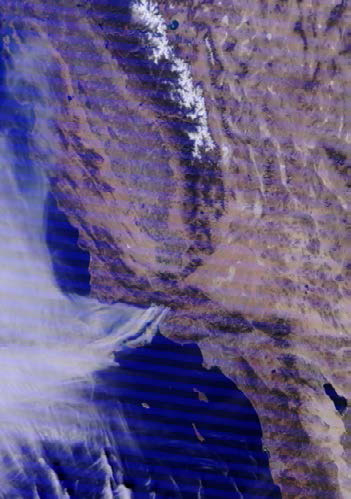
The Thomas Fire started on December 4 near Thomas Aquinas College just north of Santa Paula in Ventura County from which it received its name. Fast-moving, it quickly reached the City of Ventura. Figure 8-5 shows a photograph of the smoke plume from a location in north Oxnard looking toward the City of Ventura. The fire began burning through the rugged Santa Ynez Mountains as it threatened several small communities along the Rincon Coast north of Ventura, expanded into the Los Padres National Forest, and reached Santa Barbara County.
The unusually strong and persistent Santa Ana winds were the largest factor in the spread of the fire. The region experienced an on-and-off Santa Ana wind event for a little over two weeks, which contributed to the Thomas Fire's persistent growth. The winds also dried out the air, resulting in extremely low humidity. Figure 8-6 presents satellite views of the Thomas Fire in Ventura and Santa Barbara Counties.
Figure 8-7 shows Santa Barbara County air quality monitoring locations. Tables 8-1 through 8-3 present daily average O3, PM10, and PM2.5 concentrations color-coded by AQI Category for December 9, 14, and 18, 2017. Fine particulate matter concentrations measured at the Santa Barbara monitor indicated unhealthy conditions on December 9 and 14. Conditions returned to moderate or better levels at all monitors by December 18, 2017. Surprisingly, O3 concentrations remained mostly in the good category throughout the period.
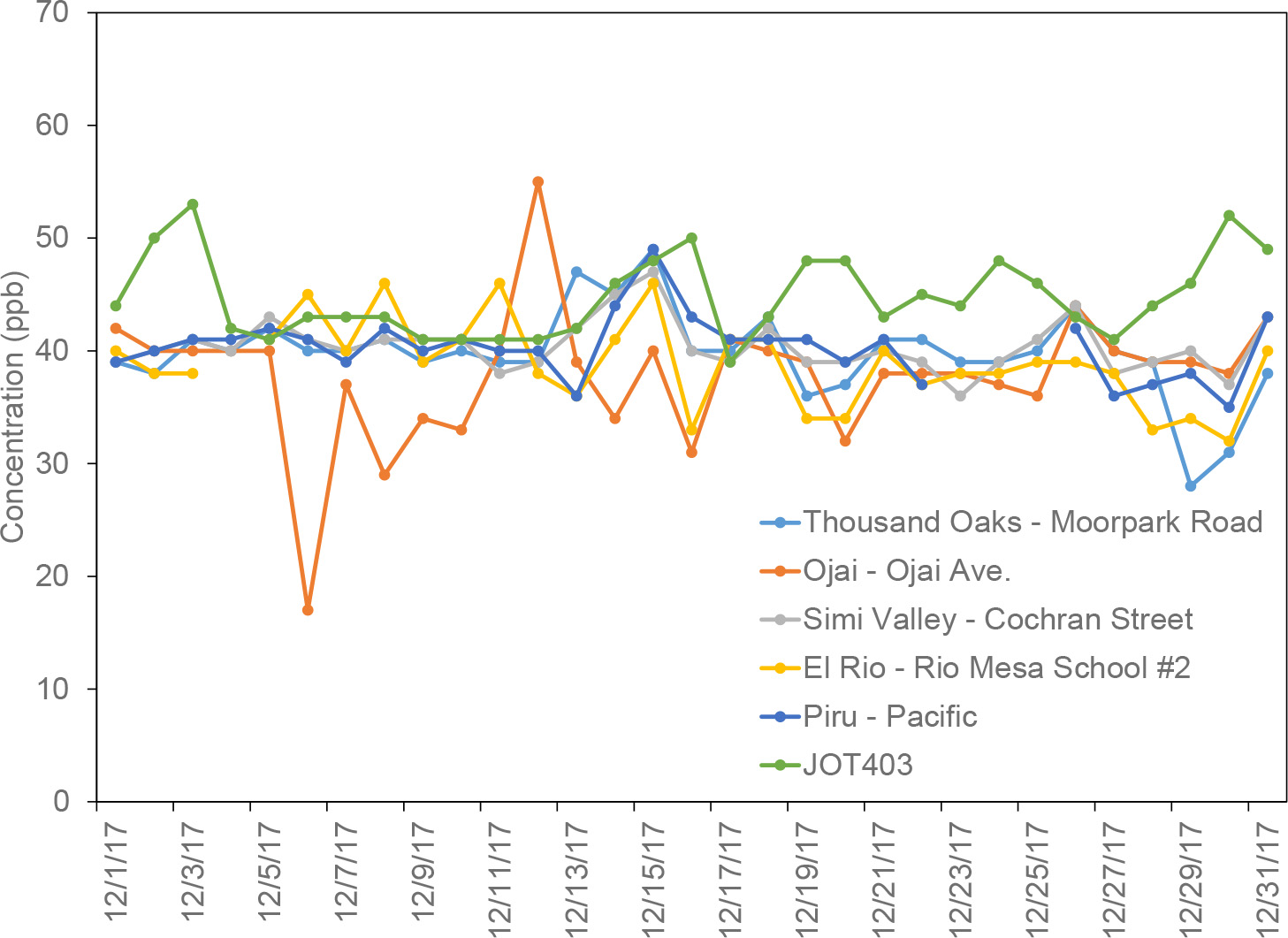
Figure 8-8 shows monitoring locations in Ventura County. Figures 8-9 and 8-10 depict PM2.5 and O3 concentrations, respectively, for five Ventura County monitors for December 2017. Figure 8-10 also shows O3 concentrations from the CASTNET site at Joshua Tree National Park (JOT403). See Figure 1-1 for the specific location. Concentrations of PM2.5 reached over 500 µg/m 3 on December 6 and 8 at Ojai at the height of the Thomas Fire. Ozone concentrations remained low during the fire. It is interesting that the lowest O3 concentration (17 ppb) at Ojai occurred during the period with the highest PM2.5 concentration (557 µg/m 3 ).
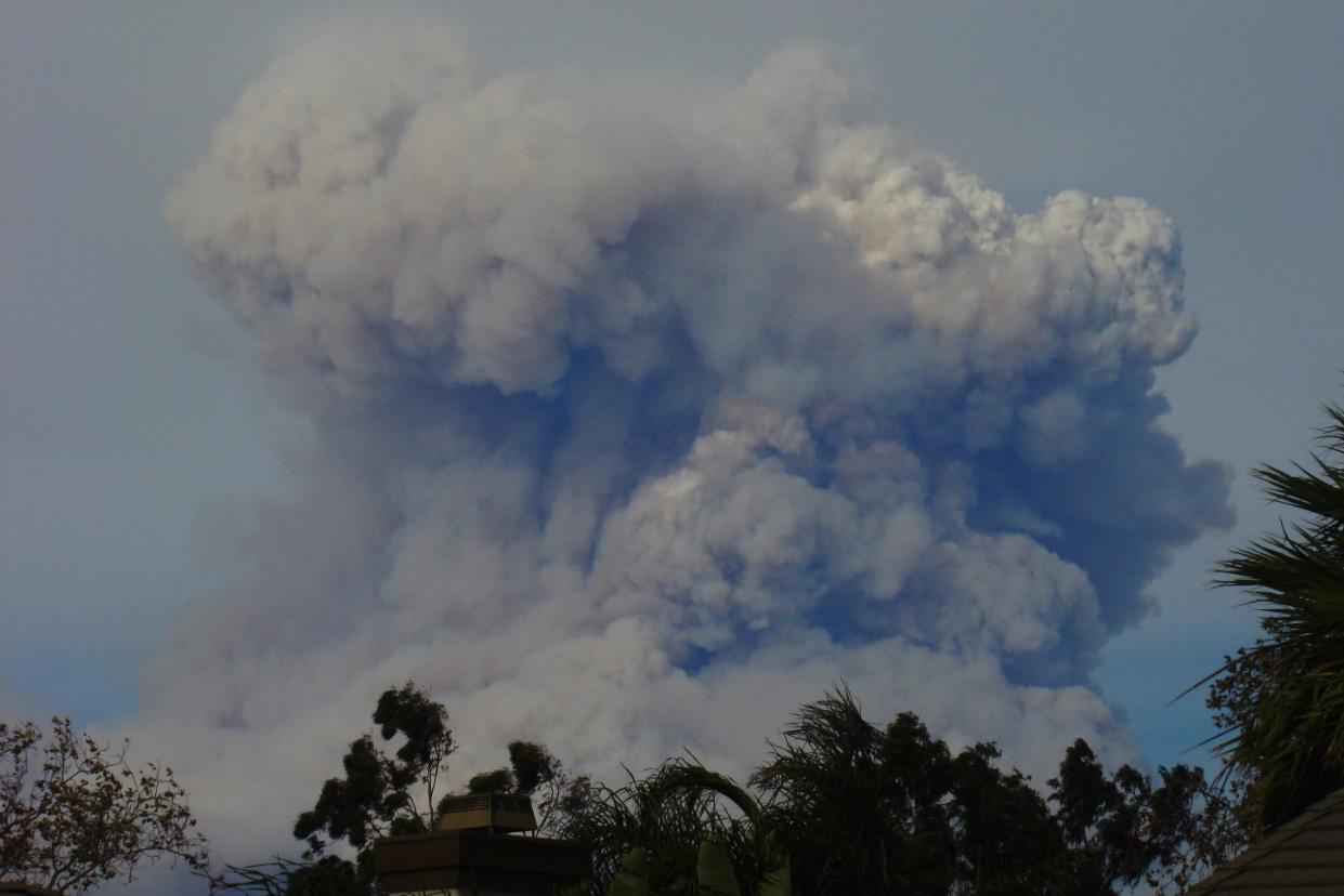
Figure 8-6 Satellite Views of the Thomas Fire in Ventura and Santa Barbara County December 5, 2017
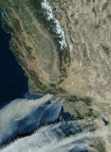
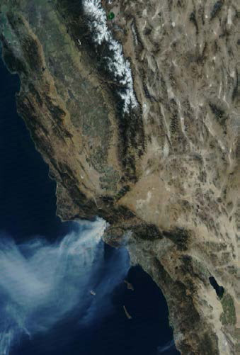
Source: National Aeronautics and Space Administration Terra satellite photo of the smoke plumes on December 5, 2017.
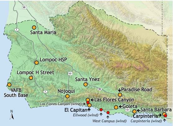
Table 8-1 Daily Average O3, PM10, and PM2.5 Concentrations by Color-Coded AQI Category for December 14, 2017
| Stations Monitoring Ozone and Particulates | |||
|---|---|---|---|
| Location | Ozone (ppb) | PM10 (µg/m) | PM2.5 (µg/m) |
| Santa Barbara | Good (10) | Unhealthy for Sensitive Groups (109) | Unhealthy (172) |
| Santa Maria | Good (27) | Good (28) | Good (48) |
| Lompoc H St | Good (18) | Moderate (53) | Moderate (96) |
| Goleta | Good (6) | Moderate (77) | Unhealthy (153) |
| El Capitan | Good (34) | Moderate (68) | |
| Las Flores Canyon | Good (43) | Moderate (59) | |
| VAFB | Good (44) | Moderate (52) | |
| Carpinteria | Good (27) | ||
| Lompoc HS and P | Good (44) | ||
| Nojoqui | Good (34) | ||
| Paradise Rd | Good (31) | ||
| Santa Ynez | Good (23) | NA | |
Source: Hoffman, 2018
Table 8-2 Daily Average O3, PM10, and PM2.5 Concentrations by Color-Coded AQI Category for December 14, 2017
| Stations Monitoring Ozone and Particulates | |||
|---|---|---|---|
| Location | Ozone (ppb) | PM10 (µg/m) | PM2.5 (µg/m) |
| Santa Barbara | Good (12) | Moderate (96) | Unhealthy (155) |
| Santa Maria | Good (26) | Good (44) | Good (43) |
| Lompoc H St | Good (24) | Good (44) | Moderate (59) |
| Goleta | Good (18) | Moderate (62) | Unhealthy for Sensitive Groups (113) |
| El Capitan | Good (39) | Moderate (52) | |
| Las Flores Canyon | Good (47) | NA | |
| VAFB | Good (48) | Moderate (51) | |
| Carpinteria | Good (19) | ||
| Lompoc HS and P | Good (49) | ||
| Nojoqui | Good (41) | ||
| Paradise Rd | Moderate (58) | ||
| Santa Ynez | Good (44) | Unhealthy for Sensitive Groups (112) | |
Source: Hoffman, 2018
Table 8-3 Daily Average O3, PM10, and PM2.5 Concentrations by Color-Coded AQI Category for December 18, 2017
| Stations Monitoring Ozone and Particulates | |||
|---|---|---|---|
| Location | Ozone (ppb) | PM10 (µg/m) | PM2.5 (µg/m) |
| Santa Barbara | Good (36) | Moderate (61) | Moderate (66) |
| Santa Maria | Good (31) | Good (45) | Good (46) |
| Lompoc H St | Good (28) | Good (49) | Moderate (53) |
| Goleta | Good (34) | Good (45) | Moderate (55) |
| El Capitan | Good (39) | Good (41) | |
| Las Flores Canyon | Good (44) | Good (47) | |
| VAFB | Good (46) | Good (49) | |
| Carpinteria | Good (34) | ||
| Lompoc HS and P | Good (44) | ||
| Nojoqui | Good (34) | ||
| Paradise Rd | Good (38) | ||
| Santa Ynez | Good (39) | Moderate (53) | |
Source: Hoffman, 2018
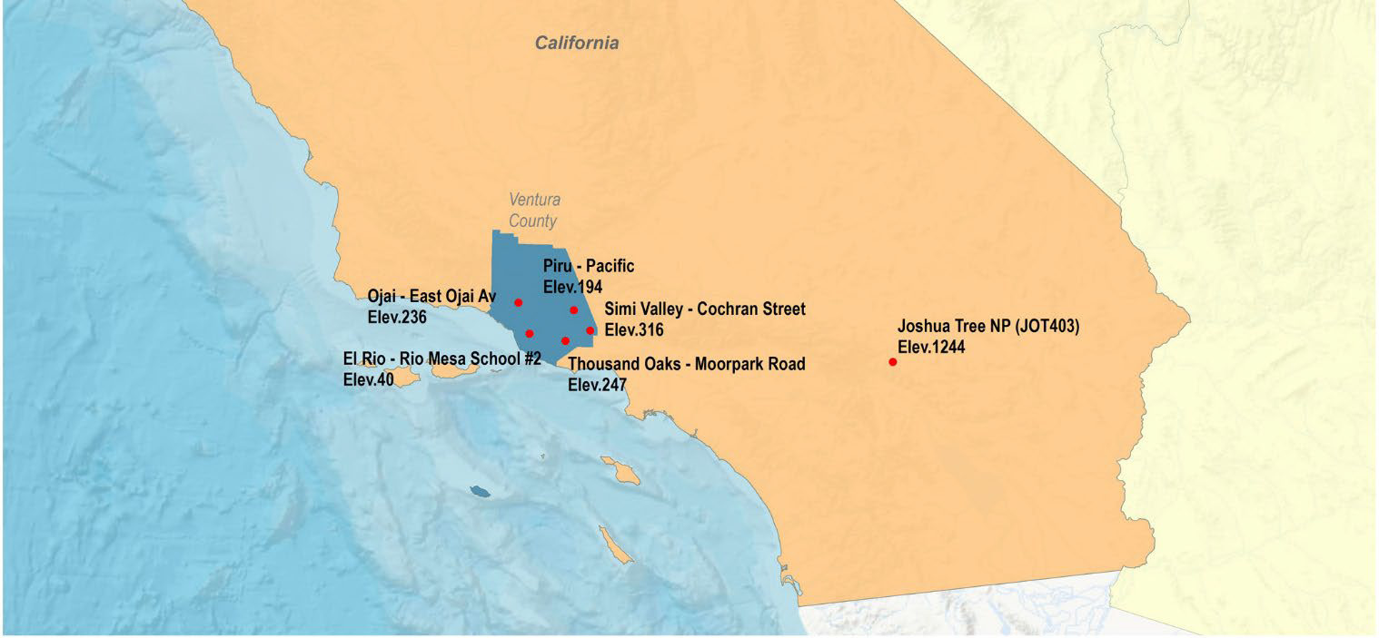
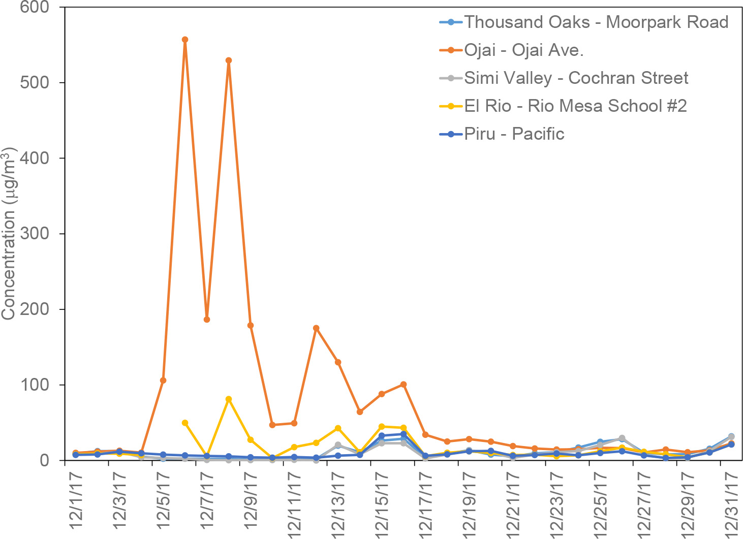
Figure 8-10 Time series of DM8A O3 Concentrations from Ventura County APCD Sites and the Joshua Tree National Park CASTNET Site (JOT403)
 Download Figure
Chapter 9: Atmospheric Deposition of Sulfur, Base Cations, and Chloride
CASTNET was designed to provide estimates of the dry deposition of nitrogen and sulfur pollutants, base cations, and chloride across the United States. EPA used the NADP TDep method to assess the status of dry and wet deposition for 2017. Total deposition was calculated as the sum of estimated dry and wet deposition.
Gaseous and particulate sulfur pollutants, base cations, and Cl - are deposited to the environment through dry and wet atmospheric processes. A principal goal of CASTNET is to estimate the rate of dry deposition of these compounds from the atmosphere to sensitive ecosystems. The NADP TDep method (EPA, 2015c; Schwede and Lear, 2014) was used to estimate dry and wet deposition. Dry and wet deposition rates were summed to obtain estimates of total deposition across the United States.
Sulfur Deposition
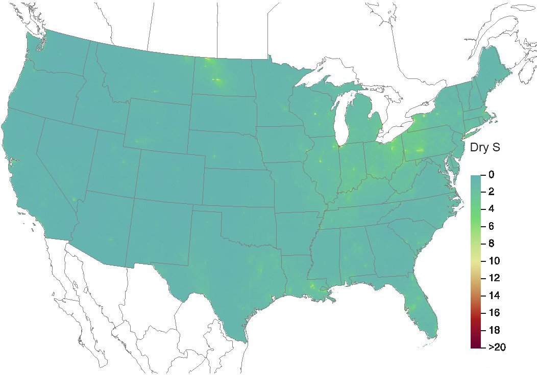
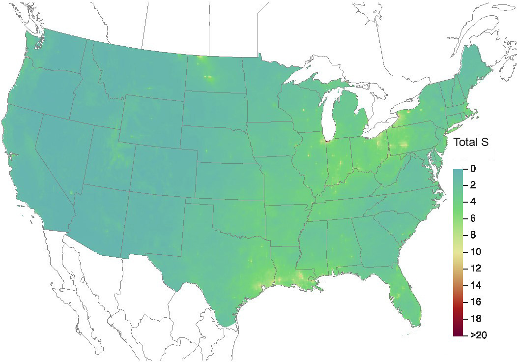
Figure 9-1 shows a map of TDep method estimates of dry deposition rates of sulfur (S) for 2017. Estimated rates of total deposition of S for 2017 are given in Figure 9-2. The magnitude of the deposition fluxes is illustrated by the shading in the figure legends. The percentage of total deposition of S due to dry deposition is shown in Figure 9-3.
Deposition of Base Cations and Chloride
A map of 2017 estimated total deposition of base cations (Ca 2+ , K + , Mg 2+ , and Na + ) is given in Figure 9-4. Figure 9-5 provides estimated rates for 2017 for total deposition of Cl -.
Figure 9-1 TDep Dry Deposition Estimates of S (kg ha -1 yr -1) for 2017
 Download Figure
Source: CASTNET|CMAQ|NADP
Figure 9-2 TDep Total Deposition Estimates of S (kg ha -1 yr -1) for 2017
 Download Figure
Source: CASTNET|CMAQ|NADP
Figure 9-3 TDep Percent of Total Deposition of S from Dry Deposition for 2017
 Download Figure
Source: CASTNET|CMAQ|NADP
Figure 9-4 TDep Total Deposition Estimates of the Base Cations Ca 2+ , K + , Mg 2+ , Na + (kiloequivalents per hectare per year) for 2017
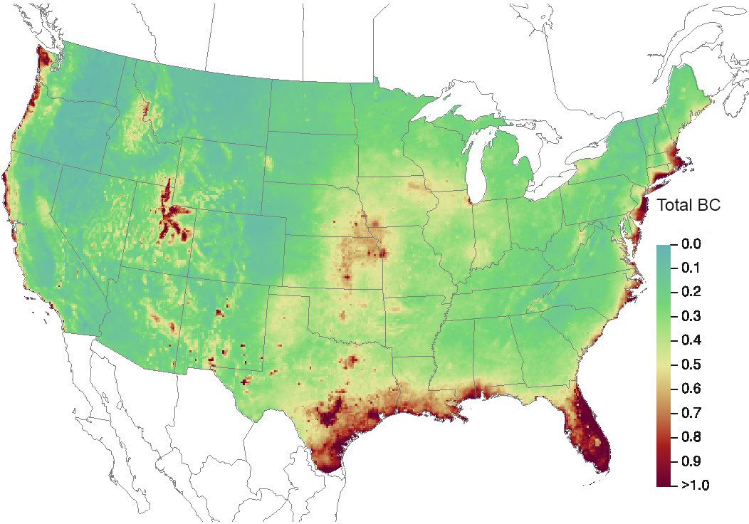 Download Figure
Source: CASTNET|CMAQ|NADP
Figure 9-5 TDep Total Deposition Estimates of Total Cl - (kg ha -1 yr -1) for 2017
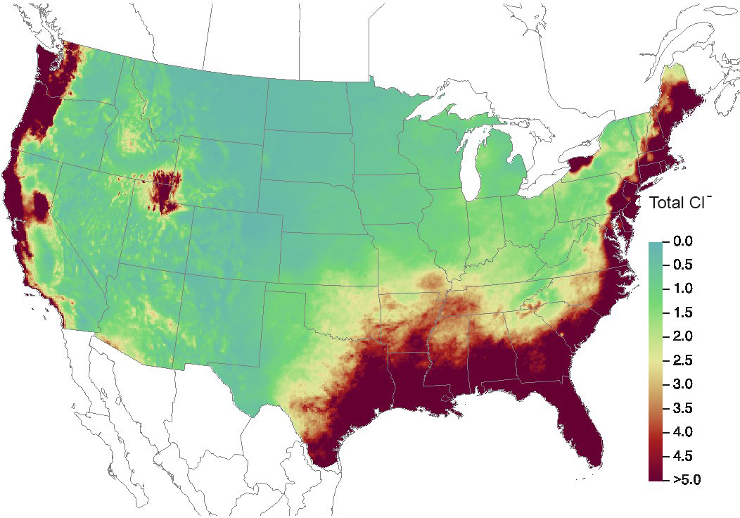 Download Figure
Source: CASTNET|CMAQ|NADP
References
Alrick, D. 2018. October 2017 Northern California Wildfires. National Air Quality Conference, Austin, January 25, 2018.
Browell, E. V., Danielsen, E. F., Ismail, S., Gregory, G. L., and Beck, S. M. (1987), Tropopause Fold Structure Determined from Airborne LIDAR and in situ Measurements, J. Geophys. Res., 92(D2), 2112–2120, doi:10.1029/JD092iD02p02112.
Byrne, K. 2018. California's 2017 Wildfire Season to Rank among Most Destructive, Costly on Record. https://www.accuweather.com/en/weather-news/californias-2017-wildfire-season-to-rank-amongmost-destructive-costly-on-record/70003704. Accessed August 2018.
Byun, D. and Schere, K. L. 2006. Review of the Governing Equations, Computational Algorithms, and Other Components of the Models-3 Community Multiscale Air Quality (CMAQ) Modeling System. Applied Mechanics Reviews, 59: 51-77. doi:10.1115/1.2128636.
CAL FIRE. 2017. Statewide Fire Summary for Monday Morning, October 30, 2017. https://goldrushcam.com/sierrasuntimes/index.php/news/local-news/11736-cal-fire-californiastatewide-fire-summary-for-monday-morning-october-30-2017-5-active-wildfires-with-around-1000-firefighters. Accessed August 2018
Danielsen, E. 1968. Stratospheric-Tropospheric Exchange Based on Radioactivity, Ozone, and Potential Vorticity. J. Atmos Sciences. Vol 25. Pages 502-518.
Danielsen, E. F., Hipskind, R. S., Gaines, S. E., Sachse, G. W., Gregory, G. L., and Hill, G. F. 1987. Three-Dimensional Analysis of Potential Vorticity Associated with Tropopause Folds and Observed Variations of Ozone and Carbon Monoxide, J. Geophys. Res., 92( D2), 2103– 2111, doi:10.1029/JD092iD02p02103.
Harshfield, G. 2018. Letter to Ozone Data Managers. Colorado Department of Public Health and Environment (CDPHE), Air Pollution Control Division (APCD). January 12.
Ho, V. and Lyons, J. 2017. Live Updates: Northern California Wildfires Cause Estimated $3 Billion Damage. San Francisco Chronicle (October 15, 2017).
Hoffman, L. 2018. Southern California Fires – December 2017. Presentation at California Air Response Planning Alliance (CARPA) 2017 Wildfire Smoke Air Response and After-Action Review.
International Organization for Standardization (ISO). 2005. Statistical Methods for the Use in Proficiency Testing by Interlaboratory Comparisons, Annex C, Robust Analysis, Section C.1: Algorithm A. Standard 13528. ISO 13528:2005(E).
Kaldunski, B., Pierce, B., and Holloway, T. 2017. When Stratospheric Ozone Hits Ground-level Regulation, Exceptional Events in Wyoming, doi:10.1175/BAMS-D-14-00133.1. Accessed August 2018.
Martin, R. S. and Baasandorj, M. 2016. A Comparison of AMoN Measurements with Localized, Arrayed Passive NH3 Samplers in Northern Utah. National Atmospheric Deposition Program (NADP), 2016 Fall Meeting, Santa Fe, NM, Oct. 31–Nov. 4.
National Oceanic and Atmospheric Administration (NOAA) National Centers for Environmental Prediction (NCEP), Weather Prediction Center. 2017. Daily Weather Map, October 9, 2017. https://www.wpc.ncep.noaa.gov/dailywxmap/index_20171009.html. Accessed August 2018.
National Oceanic and Atmospheric Administration (NOAA) Earth System Research Laboratory. 2018. The High Resolution Rapid Refresh (HRRR). https://rapidrefresh.noaa.gov/hrrr/. Accessed August 2018.
Peltier, R. E. 2017. The Hazards of Breathing Wildfire Smoke. https://www.psmag.com/environment/healthhazards-of-breathing-wildfire. Accessed September 2018.
Schwede, D. B. and Lear, G. G. 2014. A Novel Hybrid Approach for Estimating Total Deposition in the United States. Atmos. Environ., 92:207-220. doi:10.1016/j.atmosenv.2014.04.008.
U.S. Environmental Protection Agency (EPA). 2018a. Clean Air Status and Trends Network Factsheet-2018. https://www3.epa.gov/castnet/docs/CASTNET-Factsheet-2018.pdf. Accessed September 2018
U.S. Environmental Protection Agency (EPA). 2018b. Guidance on the Preparation of Exceptional Events Demonstrations for Stratospheric Ozone Intrusions. Publication No. EPA-457/B-18-001. https://nepis.epa.gov/Exe/ZyPDF.cgi/P100WS4X.PDF?Dockey=P100WS4X.PDF Accessed June 2019.
U.S. Environmental Protection Agency (EPA). 2016. Treatment of Air Quality Data Influenced by Exceptional Events. https://www.epa.gov/air-quality-analysis/treatment-air-quality-data-influenced-exceptionalevents. June 2018.
U.S. Environmental Protection Agency (EPA). 2015a. Interpretation of the Primary and Secondary National Ambient Air Quality Standards for Ozone. Title 40 Code of Federal Regulations (CFR) Appendix U to Part 50. https://www.ecfr.gov/cgi-bin/textidx?SID=9b5c394e6ac7be772c8f605a6554e08b&mc=true&node=pt40.2.50&rgn=div5#ap40.2.50_1 19.u. Accessed August 2018.
U.S. Environmental Protection Agency (EPA). 2015b. Title 40 Code of Federal Regulations (CFR) Part 50, Primary and Secondary National Ambient Air Quality Standards. https://www.ecfr.gov/cgi-bin/textidx?SID=b67492f51b28e27bf9b4226033416c93&mc=true&node=pt40.2.50&rgn=div5. Accessed August 2018.
U.S. Environmental Protection Agency (EPA). 2015c. Total Deposition Estimates Using a Hybrid Approach. ftp://ftp.epa.gov/castnet/tdep/Total_Deposition_Documentation_current.pdf. Accessed August 2018.
U.S. Environmental Protection Agency (EPA). 2014. National Emissions Inventory (NEI) Data. https://www.epa.gov/air-emissions-inventories/2014-national-emissions-inventory-nei-data Accessed August 2018.
Ute Indian Tribe of the Unitah and Ouray Reservation. 2016. Ozone NAAQS Exceedances Occurring June 8 and 9, 2015, Uinta Basin of Utah. Submitted to U.S. Environmental Protection Agency (EPA), Region 8, August 30,.
Wood Environment & Infrastructure Solutions, Inc. (Wood)*. 2017. Clean Air Status and Trends Network (CASTNET) Quality Assurance Project Plan (QAPP) Revision 9.0. Prepared for U.S. Environmental Protection Agency (EPA), Office of Air and Radiation, Clean Air Markets Division, Washington, DC. Contract No. EP-W-09-028. Gainesville, FL. http://java.epa.gov/castnet/documents.do.
Xing, J., Mathur, R., Pleim, J., Hogrefe, C., Wang, J., Gan, C.-M., Sarwar, G., Wong, D. C., and McKeen, S. 2016. Representing the Effects of Stratosphere–troposphere Exchange on 3-D O 3 Distributions in Chemistry Transport Models using a Potential Vorticity-based Parameterization, Atmos. Chem. Phys., 16, 10865-10877, https://doi.org/10.5194/acp-16-10865-2016.
Youden, W.J. (Ku, H.H., ed). 1969. Precision Measurement and Calibration. NBS Special Publication 300-Volume 1. U.S. Government Printing Office, Washington, DC.
* Formerly known as Amec Foster Wheeler Environment & Infrastructure, Inc.
Appendix A: Locational and Operational Characteristics of CASTNET Sites
| Site ID | Site Name | Start date | Latitude | Longitude | Elevation | Nearby NADP | Land Use | Terrain | Agency | Reference |
|---|---|---|---|---|---|---|---|---|---|---|
| ABT147, CT | Abington | 12/28/1993 | 41.8405 | -72.0104 | 202 | CT15 | Urban/ Agric |
Rolling | EPA | |
| ACA416, ME | Acadia NP | 12/1/1998 | 44.3771 | -68.2608 | 158 | ME98 | Forest | Rolling | NPS | |
| ALC188, TX | Alabama- Coushatta |
4/6/2004 | 30.7016 | -94.674 | 105 | TX10 | Prairie | Rolling | EPA | |
| ALH157, IL | Alhambra | 6/28/1988 | 38.869 | -89.6228 | 164 | IL46 | Agric | Flat | EPA | E |
| ANA115, MI | Ann Arbor | 6/28/1988 | 42.4166 | -83.9022 | 266 | MI52 | Forest | Flat | EPA | E |
| ARE128, PA | Arendtsville | 6/28/1988 | 39.9232 | -77.3079 | 266 | PA00 | Agric | Rolling | EPA | E |
| ASH135, ME | Ashland | 12/20/1988 | 46.6038 | -68.4132 | 231 | ME00 | Agric | Flat | EPA | E |
| BAS601, WY | Basin | 11/6/2012 | 44.28 | -108.0411 | 1242 | MT00 | Prairie | Rolling | BLM | |
| BBE401, TX | Big Bend NP | 7/18/1995 | 29.3027 | -103.1778 | 1052 | TX04 | Forest | Complex | NPS | W |
| BEL116, MD | Beltsville | 11/1/1988 | 39.0282 | -76.8171 | 47 | MD99 | Range | Flat | EPA | E |
| BFT142, NC | Beaufort | 12/28/1993 | 34.8847 | -76.6207 | 5 | NC06 | Agric | Flat | EPA | |
| BUF603, WY | Buffalo | 11/6/2012 | 44.1442 | -106.1089 | 1324 | WY99 | Prairie | Rolling | BLM | |
| BVL130, IL | Bondville | 2/9/1988 | 40.052 | -88.3725 | 213 | IL11 | Agric | Flat | EPA | E |
| BWR139, MD | Blackwater NWR |
7/4/1995 | 38.445 | -76.1113 | 1 | MD15 | Forest/ Marsh |
Coastal | EPA | |
| CAD150, AR | Caddo Valley | 10/4/1988 | 34.1793 | -93.0988 | 78 | AR03 | Forest | Complex | EPA | E |
| CAN407, UT | Canyonlands NP |
1/24/1995 | 38.4583 | -109.8213 | 1809 | UT09 | Desert | Complex | NPS | W |
| CAT175, NY | Claryville | 5/10/1994 | 41.9423 | -74.552 | 754 | NY68 | Forest | Complex | EPA | |
| CDR119, WV | Cedar Creek | 11/10/1987 | 38.8795 | -80.8477 | 240 | WV05 | Forest | Complex | EPA | E |
| CDZ171, KY | Cadiz | 1/5/1999 | 36.7841 | -87.8502 | 190 | KY99 | Agric | Rolling | EPA | |
| CHA467, AZ | Chiricahua NM |
4/25/1989 | 32.0094 | -109.3891 | 1570 | AZ98 | Range | Complex | NPS | W |
| CHC432, NM | Chaco Culture NHP |
3/1/2017 | 36.035 | -107.9042 | 1965 | CO99 | Desert | Complex | NPS | |
| CHE185, OK | Cherokee Nation |
4/2/2002 | 35.7508 | -94.6698 | 305 | AR27 | Agric | Rolling | EPA | |
| CKT136, KY | Crockett | 8/24/1993 | 37.9215 | -83.0663 | 376 | KY35 | Agric | Rolling | EPA | |
| CND125, NC | Candor | 9/25/1990 | 35.2633 | -79.8375 | 172 | NC36 | Forest | Rolling | EPA | E |
| CNT169, WY | Centennial | 5/9/1989 | 41.3645 | -106.24 | 3175 | WY95 | Forest | Complex | EPA | W |
| COW137, NC | Coweeta | 11/4/1987 | 35.0605 | -83.4303 | 683 | NC25 | Forest | Complex | EPA | E |
| CTH110, NY | Connecticut Hill |
9/29/1987 | 42.4009 | -76.6535 | 511 | NY67 | Forest | Rolling | EPA | E |
| CVL151, MS | Coffeeville | 12/27/1988 | 34.0027 | -89.7992 | 138 | MS30 | Forest | Rolling | EPA | |
| DCP114, OH | Deer Creek | 9/28/1988 | 39.6359 | -83.2606 | 264 | OH54 | Agric | Rolling | EPA | E |
| DEN417, AK | Denali NP | 10/6/1998 | 63.7232 | -148.9676 | 661 | AK03 | Forest | Complex | NPS | |
| DIN431, UT | Dinosaur NM |
11/20/2013 | 40.4373 | -109.3046 | 1463 | CO15 | Desert | Complex | NPS | |
| DUK008, NC | Duke Forest | 4/3/2017 | 35.9745 | -79.099 | 164 | NC41 | Forest | Rolling | EPA | |
| EGB181, ON | Egbert | 12/27/1994 | 44.2311 | -79.7831 | 227 | NY10 | Agric | Rolling | EPA | |
| ESP127, TN | Edgar Evins |
3/22/1988 | 36.0389 | -85.7331 | 302 | KY10 | Forest | Rolling | EPA | E |
| EVE419, FL | Everglades NP |
10/6/1998 | 25.3912 | -80.6808 | 2 | FL11 | Forest/ Marsh |
Flat | NPS | |
| FOR605, WY | Fortification Creek |
5/21/2013 | 44.3395 | -105.9198 | 1408 | WY99 | Prairie | Rolling | BLM | |
| GAS153, GA | Georgia Station |
6/28/1988 | 33.1812 | -84.4101 | 265 | GA41 | Agric | Rolling | EPA | E |
| GLR468, MT | Glacier NP | 12/27/1988 | 48.5103 | -113.9968 | 976 | MT05 | Forest | Complex | NPS | W |
| GRB411, NV | Great Basin NP |
5/16/1995 | 39.0051 | -114.2159 | 2060 | NV05 | Forest | Complex | NPS | W |
| GRC474, AZ | Grand Canyon NP |
5/16/1989 | 36.0586 | -112.1836 | 2073 | AZ03 | Forest | Rolling | NPS | W |
| GRS420, TN | Great Smoky NP- Look Rock |
10/16/1998 | 35.6335 | -83.9416 | 793 | TN11 | Forest | Complex | NPS | |
| GTH161, CO | Gothic | 5/16/1989 | 38.9563 | -106.9859 | 2915 | CO10 | Range | Complex | EPA | W |
| HOW191, ME | Howland Ameriflux |
9/27/2011 | 45.204 | -68.74 | 68 | ME09 | Forest | Rolling | EPA | |
| HOX148, MI | Hoxeyville | 10/31/2000 | 44.1809 | -85.739 | 297 | MI53 | Forest | Flat | EPA | |
| HWF187, NY | Huntington Wildlife Forest |
5/28/2002 | 43.973 | -74.2233 | 497 | NY20 | Forest | Complex | EPA | |
| IRL141, FL | Indian River Lagoon |
7/9/2001 | 27.8492 | -80.4556 | 2 | FL99 | Coastal/ Marsh | Flat/ Water | EPA | |
| JOT403, CA | Joshua Tree NP | 2/16/1995 | 34.0696 | -116.3889 | 1244 | CA67 | Desert | Complex | NPS | W |
| KEF112, PA | Kane Experimental Forest |
1/3/1989 | 41.5981 | -78.7679 | 618 | PA29 | Forest | Rolling | EPA | E |
| KIC003, KS | Kickapoo Tribe |
2/18/2014 | 39.8539 | -95.6578 | 367 | KS97 | Prairie | Rolling | EPA | |
| KNZ184, KS | Konza Prairie |
3/26/2002 | 39.1022 | -96.6096 | 346 | KS31 | Prairie | Flat | EPA | |
| LAV410, CA | Lassen Volcanic NP |
7/25/1995 | 40.54 | -121.5765 | 1756 | CA96 | Forest | Complex | NPS | W |
| LRL117, PA | Laurel Hill |
12/15/1987 | 39.9883 | -79.2516 | 609 | PA83 | Forest | Complex | EPA | E |
| MAC426, KY | Mammoth Cave NP |
7/24/2002 | 37.1314 | -86.1481 | 243 | KY10 | Agric | Rolling | NPS | |
| MCK131, KY | Mackville | 7/31/1990 | 37.7047 | -85.0487 | 293 | KY03 | Agric | Rolling | EPA | E |
| MCK231, KY | Mackville Co-located |
12/29/1992 | 37.7047 | -85.0487 | 293 | KY03 | Agric | Rolling | EPA | |
| MEV405, CO | Mesa Verde NP |
1/10/1995 | 37.1984 | -108.4905 | 2165 | CO99 | Forest | Complex | NPS | W |
| MKG113, PA | M.K. Goddard |
1/12/1988 | 41.4268 | -80.1452 | 377 | NY10 | Forest | Rolling | EPA | E |
| NEC602, WY | Newcastle | 11/7/2012 | 43.873 | -104.1919 | 1468 | WY99 | Prairie | Rolling | BLM | |
| NIC001, NY | Nicks Lake | 11/20/2012 | 43.6805 | -74.9891 | 525 | NY29 | Forest | Rolling | NYSDEC | |
| NPT006, ID | Nez Perce Tribe |
12/15/2015 | 46.2756 | -116.0216 | 945 | Forest | Rolling | EPA | ||
| OXF122, OH | Oxford | 8/18/1987 | 39.5311 | -84.7235 | 284 | OH09 | Agric | Rolling | EPA | E |
| PAL190, TX | Palo Duro SP |
4/24/2007 | 34.8806 | -101.6647 | 1053 | TX02 | Prairie | Complex | EPA | |
| PAR107, WV | Parsons | 1/19/1988 | 39.0904 | -79.6617 | 510 | WV18 | Forest | Complex | EPA | E |
| PED108, VA | Prince Edward |
11/3/1987 | 37.1652 | -78.3071 | 149 | VA24 | Forest | Rolling | EPA | E |
| PET427, AZ | Petrified Forest |
9/12/2002 | 34.8225 | -109.8925 | 1723 | AZ97 | Desert | Flat | NPS | |
| PIN414, CA | Pinnacles NM |
5/16/1995 | 36.4832 | -121.1569 | 335 | CA66 | Forest | Complex | NPS | W |
| PND165, WY | Pinedale | 12/27/1988 | 42.929 | -109.7878 | 2386 | WY06 | Forest | Rolling | EPA | W |
| PNF126, NC | Cranberry | 12/27/1988 | 36.1054 | -82.045 | 1216 | NC45 | Forest | Mountain-top | EPA | E |
| PRK134, WI | Perkinstown | 9/27/1988 | 45.2065 | -90.5972 | 462 | WI35 | Agric | Rolling | EPA | E |
| PSU106, PA | Penn State | 1/6/1987 | 40.7209 | -77.9318 | 364 | PA42 | Agric | Rolling | EPA | E |
| QAK172, OH | Quaker City | 1/5/1999 | 39.9427 | -81.3379 | 371 | OH49 | Agric | Rolling | EPA | |
| RED004, MN | Red Lake Nation |
8/26/2014 | 47.8638 | -94.8352 | 372 | MN16 | Forest | Flat | EPA | |
| ROM206, CO | Rocky Mountain NP Co-located |
7/3/2001 | 40.2781 | -105.5456 | 2742 | CO19 | Forest | Complex | EPA | |
| ROM406, CO | Rocky Mountain NP |
12/20/1994 | 40.2781 | -105.5456 | 2743 | CO19 | Forest | Complex | NPS | W |
| SAL133, IN | Salamonie Reservoir |
6/28/1988 | 40.816 | -85.6614 | 250 | IN20 | Agric | Flat | EPA | E |
| SAN189, NE | Santee Sioux |
7/5/2006 | 42.8292 | -97.8541 | 434 | SD99 | Range | Rolling | EPA | |
| SEK430, CA | Sequoia & Kings Canyon NP- Ash Mountain |
4/7/2005 | 36.4895 | -118.8292 | 510 | CA75 | Forest | Mountain-top | NPS | |
| SHE604, WY | Sheridan | 11/6/2012 | 44.93 | -106.85 | 1115 | MT00 | Prairie | Rolling | BLM | |
| SHN418, VA | Shenandoah NP - Big Meadows |
6/28/1988 | 38.5231 | -78.4347 | 1073 | VA28 | Forest | Mountain-top | NPS | E |
| SND152, AL | Sand Mountain |
12/27/1988 | 34.289 | -85.9701 | 349 | AL99 | Agric | Rolling | EPA | E |
| SPD111, TN | Speedwell | 6/12/1989 | 36.4698 | -83.8265 | 361 | TN04 | Agric | Rolling | EPA | E |
| STK138, IL | Stockton | 12/28/1993 | 42.2872 | -90 | 281 | IL18 | Agric | Rolling | EPA | |
| SUM156, FL | Sumatra | 12/27/1988 | 30.1102 | -84.9904 | 16 | FL23 | Forest | Flat | EPA | E |
| THR422, ND | Theodore Roosevelt NP |
10/6/1998 | 46.8948 | -103.3777 | 850 | ND00 | Forest | Rolling | NPS | |
| UND002, VT | Underhill | 11/13/2012 | 44.5283 | -72.8688 | 399 | VT99 | Forest | Complex | EPA | |
| UVL124, MI | Unionville | 6/28/1988 | 43.6136 | -83.3599 | 202 | MI51 | Agric | Flat | EPA | E |
| VIN140, IN | Vincennes | 8/4/1987 | 38.7408 | -87.4849 | 136 | IN22 | Agric | Rolling | EPA | E |
| VOY413, MN | Voyageurs NP | 6/13/1996 | 48.4125 | -92.8292 | 429 | MN32 | Forest | Rolling | NPS | |
| VPI120, VA | Horton Station |
6/2/1987 | 37.3298 | -80.5575 | 920 | VA13 | Agric | Mountain-top | EPA | E |
| WFM007, NY | Whiteface Mountain Summit |
6/4/2015 | 44.36608 | -73.90312 | 1415 | NY98 | Forest | Complex | EPA | |
| WFM105, NY | Whiteface Mountain |
11/20/2012 | 44.39 | -73.86 | 570 | NY98 | Forest | Complex | NYSDEC | |
| WNC429, SD | Wind Cave NP |
11/20/2003 | 43.5576 | -103.4839 | 1292 | SD04 | Prairie | Rolling | NPS | |
| WSP144, NJ | Washington Crossing |
12/27/1988 | 40.3123 | -74.8727 | 59 | NJ99 | Range | Rolling | EPA | E |
| WST109, NH | Woodstock | 12/27/1988 | 43.9445 | -71.7008 | 255 | NH02 | Forest | Complex | EPA | E |
| YEL408, WY | Yellowstone NP | 6/26/1996 | 44.5654 | -110.4003 | 2400 | WY08 | Agric | Rolling | NPS | W |
| YOS404, CA | Yosemite NP - Turtleback Dome |
9/25/1995 | 37.7133 | -119.7062 | 1605 | CA99 | Forest | Complex | NPS | W |
Note:
NM = National Monument
NP = National Park
NWR = National Wildlife Reserve
SP = State Park
E = eastern reference site
W = western reference site
Appendix B: Acronyms and Abbreviations
| A2LA | American Association for Laboratory Accreditation |
| AJAX | Alpha Jet Atmospheric eXperiment |
| AMNet | Atmospheric Mercury Network |
| AMoN | Ammonia Monitoring Network |
| APCD | air pollution control district |
| AQI | air quality index |
| AQS | EPA's Air Quality System |
| ARP | Acid Rain Program |
| BLM | Bureau of Land Management |
| °C | degrees Celsius |
| Ca | particulate calcium |
| CAPMoN | Canadian Air and Precipitation Monitoring Network |
| CASTNET | Clean Air Status and Trends Network |
| CDPHE | Colorado Department of Public Health and the Environment |
| CFR | Code of Federal Regulations |
| Cl - | particulate chloride |
| CMAQ | Community Multiscale Air Quality Modeling System |
| CO | carbon monoxide |
| DM8A | daily maximum 8-hour average |
| DQI | data quality indicator |
| ECAN | Environment Canada |
| EGUs | electric generating units |
| EPA | U.S. Environmental Protection Agency |
| GOES | Geostationary Operational Environmental Satellite system |
| hPa | hectopascal |
| HNO | nitric acid |
| IMPROVE | Interagency Monitoring of Protected Visual Environments |
| IO | informational stratospheric intrusion data flags |
| ISO | International Organization for Standardization |
| K | Kelvin |
| K + | particulate potassium |
| kg | kilogram |
| kg ha -1 yr -1 | kilograms per hectare per year |
| m | meter |
| m 2/sec | square meter per second |
| MARPD | mean absolute relative percent difference |
| mb | millibar |
| MDN | Mercury Deposition Network |
| MERRA-2 | Modern-Era Retrospective Analysis for Research and Applications, Version 2 |
| Mg 2+ | particulate magnesium |
| MST | Mountain Standard Time |
| N | nitrogen |
| Na + | particulate sodium |
| NAAQS | National Ambient Air Quality Standards |
| NADP | National Atmospheric Deposition Program |
| NAM | North American Mesoscale model |
| NCore | EPA's National Core Monitoring |
| NH3 | ammonia |
| NH4+ | particulate ammonium |
| NO | nitrogen dioxide |
| NO3- | particulate nitrate |
| NOx | nitrogen oxides [nitrogen oxide (NO) + nitrogen dioxide (NO2)] |
| NOy | total reactive oxides of nitrogen |
| NOAA | National Oceanic and Atmospheric Administration |
| NPS | National Park Service |
| NTN | National Trends Network |
| O3 | ozone |
| PM2.5 | fine particulate matter |
| PM10 | particulate matter with a mean aerodynamic diameter less than 10 micrometers |
| ppb | parts per billion |
| ppm | parts per million |
| PRISM | Parameter-elevation Regressions on Independent Slopes Model |
| PT | proficiency testing |
| PV | potential vorticity |
| PVU | potential vorticity unit (m 2/sec times Kelvin/kilogram) |
| QA | quality assurance |
| QAPP | Quality Assurance Project Plan |
| RAP | Rapid Refresh Model |
| RAQMS | Realtime Air Quality Modeling System |
| S | sulfur |
| SI Workgroup | EPA Ozone Stratospheric Intrusion Workgroup |
| SO2 | sulfur dioxide |
| SO42- | particulate sulfate |
| TDEP | NADP Total Deposition Hybrid Method |
| total NO3- | gaseous nitric acid (HNO) + particulate nitrate (NO) |
| µg/m 3 | micrograms per cubic meter |
| WARMS | Wyoming Air Resources Monitoring System |
| WDEQ/AQD | State of Wyoming Department of Environmental Quality/Air Quality Division |