Executive Summary
The EPA Clean Air Status and Trends Network (CASTNET) measures concentrations of atmospheric pollutants across the United States. The primary objectives of the network are to determine compliance with ozone National Ambient Air Quality Standards and to provide data to evaluate the effectiveness of national and regional air pollution control programs. CASTNET data are also used to provide input to the National Atmospheric Deposition Program’s Total Deposition Hybrid Method for calculating total deposition and evaluating regional air quality models. This report presents maps of 2016 ozone levels, nitrogen and sulfur pollutant concentrations, and deposition fluxes and examines trends in air quality over the 27-year period from 1990 through 2016. In 2016, CASTNET measured rural, regionally representative concentrations of nitrogen and sulfur species at 95 monitoring stations at 93 locations and ozone levels at 81 locations.
Key Results and Highlights through 2016
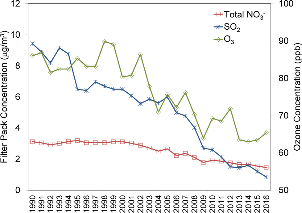
The median fourth highest daily maximum 8-hour average (DM8A) ozone (O3) concentration for 2016 at the eastern CASTNET reference sites (see Appendix A for designated reference sites) was 64 parts per billion (ppb). This is a slight increase from the 2015 median of 63.5 ppb. At the western CASTNET reference sites, the median was 66 ppb. Three-year averages of fourth highest DM8A O3 concentrations exceeded the 2015 8-hour National Ambient Air Quality Standard (NAAQS) of 0.070 parts per million (ppm) or, equivalently, 70 ppb, at three California CASTNET sites and one site in New Jersey during the most recent 3 year period (2014–2016). During 2016, 10 eastern, 4 California sites, and Dinosaur National Monument (DIN431), UT measured fourth highest DM8A O3 concentrations greater than 70 ppb. Three-year averages of fourth highest DM8A O3 concentrations have been reduced by 24 percent at the eastern reference sites since 1990–1992 and by 10 percent at the western reference sites since 1996–1998. Figure E-1 and Table E-1 summarize the long-term changes in measured concentrations.
Regional O3 concentrations are influenced by nitrogen oxides (NOx) emissions. Federal, state, and local NOx control programs have resulted in substantive reductions in emissions. For example, NOx emissions declined by 86 percent over the 27 year period, 1990 through 2016, at regulated electric generating units (EGUs) in the East.
Three-year mean annual concentrations of total nitrate (NO3-), which is comprised of nitric acid plus particulate NO3-, declined 48 percent at the eastern reference sites over the 27-year period. Three-year mean annual total NO3- levels measured at the western reference sites dropped by 34 percent over the 21-year period.
Mean annual sulfur dioxide (SO2) concentrations measured at the eastern reference sites have declined significantly over the 27-year period, 1990 through 2016. Three-year mean annual SO2 levels at eastern sites decreased 86 percent. SO2 concentrations measured at the western reference sites declined by 46 percent over the 20 years from 1996 through 2016.
The percent reduction in SO2 concentrations at the eastern reference sites is consistent with the reduction in regulated eastern EGU SO2 emissions (94 percent).
Table E-1 Trends in Aggregated Western and Eastern O3, Total NO3-, and SO2 Pollutant Concentrations
| Pollutant | Western Reference Sites | Eastern Reference Sites | Percent Changed | |||
|---|---|---|---|---|---|---|
| 1996-1998 | 2014-2016 | 1990-1992 | 2014-2016 | West | East | |
| O3 (ppb) | 74 | 66 | 85 | 64 | -10 | -24 |
| Total NO3- (µg/m 3 ) | 1.0 | 0.7 | 3.0 | 1.6 | -34 | -48 |
| SO2 (µg/m 3 ) | 0.6 | 0.3 | 8.8 | 1.2 | -46 | -86 |
The original intent of CASTNET was to measure pollutant concentrations to estimate trends in sulfur and nitrogen pollutants. Currently, the focus also includes demonstrating compliance of rural, regional O3 concentrations with the NAAQS. The network also features measurements of trace-level gases and speciated nitrogen pollutants. Additionally, CASTNET supports the National Atmospheric Deposition Program’s Ammonia Monitoring Network with operation of ammonia samplers at 69 CASTNET sites. This report provides information on CASTNET pollutant measurements, estimated deposition fluxes, and other topics that can be addressed using CASTNET data, such as wintertime ozone concentrations in the Uinta Basin, Utah, effects of wildfires on air quality in Wyoming and Arizona, and pollutant concentrations measured on Whiteface Mountain, New York.
Chapter 1: CASTNET Update
The Clean Air Status and Trends Network (CASTNET) is a nationwide air quality monitoring network that began operating in 1991. The network provides measurements of air pollutant concentrations in rural areas across the United States over the long term to determine compliance with ozone National Ambient Air Quality Standards and to evaluate the effectiveness of national and regional emission control programs. CASTNET data are used to provide input to regional air quality models. CASTNET is managed and operated by the U.S. Environmental Protection Agency in cooperation with the National Park Service and other federal, state, tribal, and local partners. In 2016, the network operated 95 monitoring stations throughout the contiguous United States, Alaska, and Canada. CASTNET data show a 27-year decline in ozone concentrations and in nitrogen and sulfur pollutant levels and deposition rates.
Introduction
The Clean Air Status and Trends Network (CASTNET) operated 95 monitoring stations throughout the contiguous United States, Alaska, and Canada in 2016. All 95 sites included filter pack systems to sample weekly concentrations of acid gases and aerosols. Eighty-one sites included continuous ozone (O3) analyzers. The U.S. Environmental Protection Agency (EPA) and the National Park Service (NPS) are the primary sponsors of CASTNET. NPS began its participation in 1994 and operated 25 sites during 2016. The Bureau of Land Management-Wyoming State Office (BLM) operated five sites in Wyoming.
CASTNET depends on contributions from many organizations (EPA, 2015a) including Native American tribes, state and federal government agencies, and universities. These participants sponsor individual CASTNET sites and provide in-kind services that support the overall performance of the network. For example, partners operate and repair site instruments, change weekly filter packs, and perform general site maintenance. Many partners provide the land for the CASTNET site. Others, such as universities, provide their expertise in air quality monitoring, which is invaluable for improving CASTNET monitoring capabilities and ensuring that CASTNET collects data that are valued by the scientific research community.
In 2016, ozone monitoring was added to the Nez Perce Tribe’s site in Idaho (NPT006), and the site was converted from off grid to normal power. The seasonal small footprint site at the summit of Whiteface Mountain, NY (WFM007) was operated by the New York State Department of Environmental Conservation (NYSDEC) during the summer of 2016. The site at Coweeta, NC (COW005) was shut down in August 2016 after completion of a special study that utilized solar and wind energy as sources of power for the small footprint site.
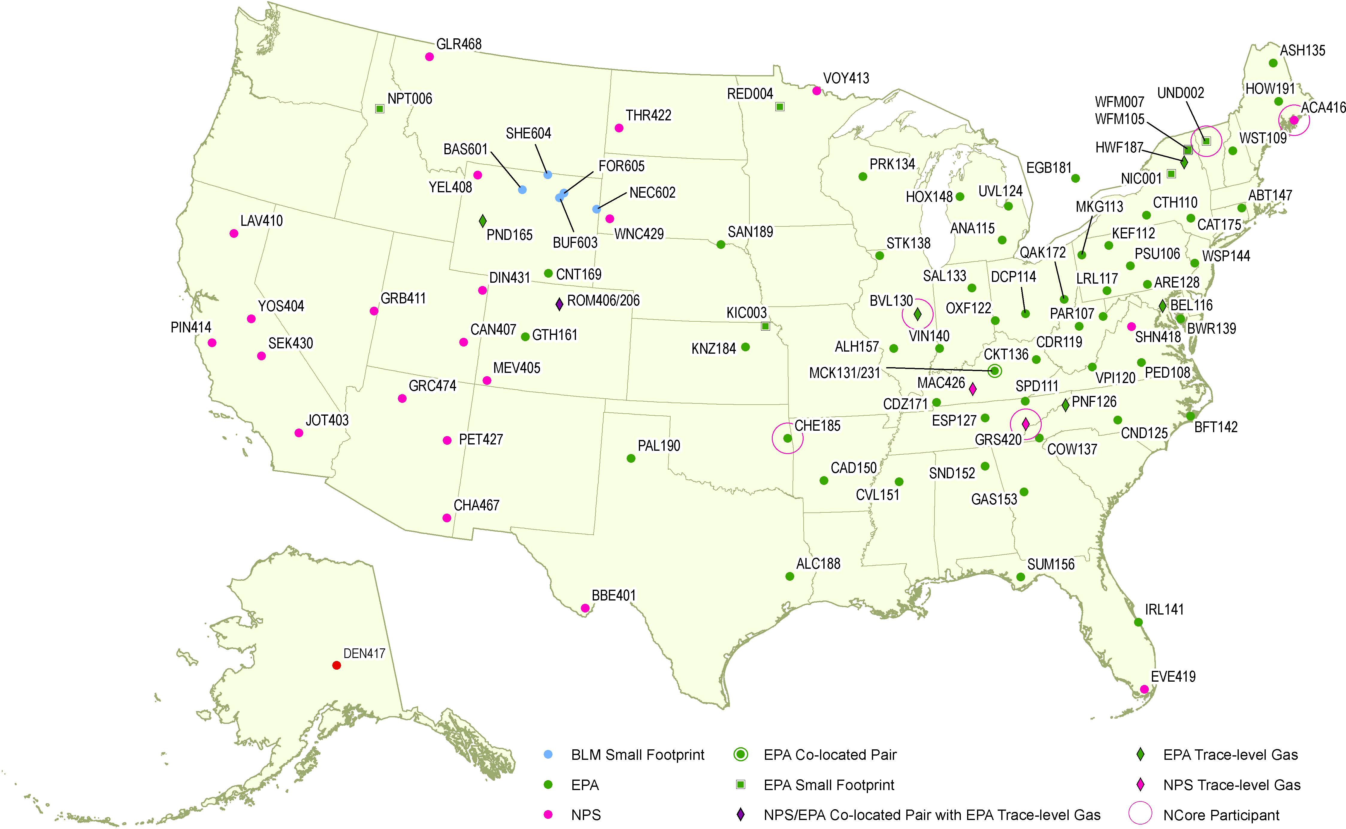
The U.S. Congress established the Acid Rain Program (ARP) in 1990 to reduce emissions of sulfur dioxide (SO2) and nitrogen oxides (NOx) from electric generating units (EGUs). Congress also directed EPA to establish CASTNET to assess the effectiveness of the ARP by providing consistent, long-term measurements for determining relationships between changes in emissions and changes in air quality, atmospheric deposition, and ecological effects. Figure 1-1 shows the locations of the CASTNET monitoring sites that were operational during 2016.
Related Air Quality Networks
CASTNET monitors air quality and deposition in cooperation with other national and international networks. EPA uses data from CASTNET and the other long-term national networks to assess the effectiveness of emission control programs. These networks include the National Atmospheric Deposition Program (NADP) and its affiliated networks:
- National Trends Network (NTN)
- Ammonia Monitoring Network (AMoN)
- Mercury Deposition Network (MDN)
- Atmospheric Mercury Network (AMNet)
Other cooperating networks include:
- Canadian Air and Precipitation Monitoring Network (CAPMoN)
- EPA’s National Core Monitoring (NCore)
- BLM’s Wyoming Air Resources Monitoring System (WARMS)
- Interagency Monitoring of Protected Visual Environments (IMPROVE)
Locations of Monitoring Sites
A map of CASTNET monitoring sites is given in Figure 1-1. Ninety-five monitoring sites were operated at 93 distinct locations. To estimate precision across the network, co-located sites were operated at Mackville, KY (MCK131/231) and Rocky Mountain National Park, CO (ROM406/206) during 2016. The ROM406/206 pair ensures consistency between EPA (ROM206) and NPS (ROM406). Of the two Rocky Mountain monitoring sites, ROM406 is specified as the regulatory monitoring site for O3. The location of each site and information on start date, latitude, longitude, elevation, identification of the nearby NADP site, land use, terrain type, operating agency, and if the site is a reference site used for trends are given in Appendix A.
Measurements Recorded at CASTNET Sites
All CASTNET sites measure weekly ambient concentrations of acidic pollutants, base cations, and chloride (Cl -) using a 3-stage filter pack with a controlled flow rate (Wood, 2015). Gaseous pollutant concentrations include nitric acid (HNO3) and SO2. Particulate concentrations include nitrate (NO3-), ammonium (NH4+), sulfate (SO42-), magnesium (Mg 2+ ), calcium (Ca 2+ ), potassium (K + ), sodium (Na + ), and Cl -. The filter pack is exchanged each Tuesday and shipped to the analytical chemistry laboratory for analysis. Ambient temperature is measured at 9 meters (m) at all sites in part to enable conversion of concentrations to local conditions.
Most CASTNET sites also include a temperature-controlled shelter and continuous O3 monitoring system. O3 concentrations were measured at 81 sites. The O3 inlet and filter pack are located atop a 10-m tower. Some CASTNET sites also measure trace-level SO2, carbon monoxide (CO), and nitrogen oxide/total reactive oxides of nitrogen (NO/NOy). In 2016, meteorological parameters were measured at 6 EPA-, 25 NPS-, and 5 BLM-sponsored CASTNET sites. Measured meteorological parameters include 2-m temperature, wind speed and direction, standard deviation of the wind direction, solar radiation, relative humidity, precipitation, and surface wetness (at select sites).
Quality Assurance Program
The CASTNET quality assurance (QA) program was established to ensure that all reported data are of known and documented quality in order to meet CASTNET objectives. The QA program also ensures intra-network consistency and comparability and the delivery of data that are reproducible and comparable with data from other monitoring networks. The 2016 QA program elements are documented in the CASTNET Quality Assurance Project Plan (QAPP; Wood, 2015). The QAPP includes standards and policies for all components of project operation, from site selection through final data reporting, with appendices that provide standard operating procedures for CASTNET operations.
Data quality indicators (DQI) such as precision, accuracy, and completeness are used to assess CASTNET measurements and supporting activities. Routine assessment and analysis help guarantee the production of high-quality data and information to meet project objectives. Measurements taken during 2016 and historical data collected over the period 1990 through 2015 were analyzed relative to DQI and their associated metrics. Results from these analyses are available in quarterly and annual QA reports posted on the EPA CASTNET website.
The Wood CASTNET laboratory regularly participates in interlaboratory comparison studies and proficiency testing (PT) programs such as the Environment Canada (ECAN) PT Program for Inorganic Environmental Substances. The ECAN PT program conforms to the requirements of the American Association for Laboratory Accreditation (A2LA). The program meets the International Organization for Standardization (ISO)/International Electrotechnical Commission (IEC) 17043:2010 conformity assessment – general requirements for proficiency testing with scope of accreditation 2867.01. The results reported are evaluated for systematic bias and precision. Systematic bias is assessed using the Youden (1969) non-parametric analysis, while precision is calculated using algorithm A from the ISO standard 13528 (ISO, 2005). CASTNET laboratory results from the PT studies are summarized in the QA quarterly and annual reports posted to the EPA CASTNET website.
Estimating Dry, Wet, and Total Deposition
Total deposition was assessed using the NADP’s Total Deposition Hybrid Method (EPA, 2015d; Schwede and Lear, 2014), which is a hybrid approach that combines data from established ambient monitoring networks and chemical transport models. To estimate dry deposition, ambient measurement data from CASTNET and other networks were merged with dry deposition rates and flux output from the Community Multiscale Air Quality (CMAQ) modeling system. Wet deposition estimates were derived from precipitation chemistry measurements and precipitation amounts from the Parameter-elevation Regressions on Independent Slopes Model (PRISM). Dry and wet deposition fluxes were added to obtain the estimates of total deposition that are discussed in Chapters 8 and 10.
This report summarizes CASTNET monitoring and the resulting concentration and deposition data collected over the 27-year period from 1990 through 2016. The report covers such topics such as wintertime air quality in the Uinta Basin in Utah, trace-level gas concentrations measured at eight CASTNET sites, effects of wildfires on air quality, and air quality on Whiteface Mountain in New York. Additional information, previous annual reports, descriptions of CASTNET operations, other CASTNET documents, and the CASTNET database can be found on the EPA CASTNET website.
Chapter 2: Ozone Concentrations
CASTNET is the principal network for monitoring rural, ground-level ozone concentrations in the United States. The network produces ozone data for evaluation of compliance with the National Ambient Air Quality Standards (NAAQS; EPA, 2015) plus information on geographic patterns in regional ozone levels. CASTNET ozone data are of the highest quality as demonstrated by the results from the CASTNET QA program and its rigorous QA/quality control procedures. Ozone data measured at 78 of 81 CASTNET sites from 2014 through 2016 were evaluated with respect to the NAAQS and used to calculate design values under Title 40 Code of Federal Regulations Part 50 Appendix U (EPA, 2015b). Maps of 3-year averages of fourth highest daily maximum 8-hour average (DM8A) ozone concentrations for 2014 through 2016 and fourth highest DM8A ozone concentrations for 2016 are presented. Trends in fourth highest DM8A ozone concentrations for eastern and western reference sites are shown. For the 2014 through 2016 period, three California sites and one eastern site measured concentrations greater than the 0.070 ppm NAAQS.
Hourly average concentrations were measured at 81 CASTNET sites in 2016. These data are archived in the CASTNET database and delivered routinely to the EPA Air Quality System (AQS) database. Data from these sites, with the exception of Howland, ME (HOW191) and the co-located sites at MCK231, KY and ROM206, CO, which are designated as non-regulatory, are used to calculate fourth highest DM8A O3 concentrations when three years of Title 40 Code of Federal Regulations (CFR) Part 58-compliant data become available. CASTNET measurements provide information for evaluating rural O3 concentrations in the context of the O3 NAAQS and in terms of presenting information on trends and geographic patterns in regional O3.
A design value describes the air quality status of a given area with respect to the concentration values required by the NAAQS. Design values change as each new 3-year period of monitored ozone concentrations becomes available (e.g., 2014–2016). Design values are used to classify nonattainment areas, assess progress towards meeting the NAAQS, and develop control strategies to achieve the NAAQS. For example, to achieve the 2015 ozone NAAQS, 3-year averages of fourth highest DM8A ozone concentrations cannot exceed 0.070 parts per million (ppm). Designated criteria pollutant nonattainment areas are provided on the EPA website.
The information presented in this chapter includes maps of and trends in the annual fourth highest DM8A O3 concentrations measured at CASTNET sites. Ozone data from Dinosaur National Monument (NM) in Utah (DIN431) and from measurements in the Uinta Basin in the northeast corner of Utah are also discussed. Additional maps of O3 concentrations from the NPS Air Atlas can be viewed at Air Atlas and Air Quality in Parks.
Measurements from 34 eastern and 16 western reference sites (see Appendix A) were analyzed to determine trends in O3 concentrations. These sites were also used to show trends in ambient nitrogen and sulfur concentrations (chapters 3 and 5). The eastern reference sites have been reporting CASTNET measurements since at least 1990 and the western reference sites since at least 1996.
2015 National Ambient Air Quality Standards for Ozone
| Ozone | Primary Standard | Secondary Standard | ||
|---|---|---|---|---|
| Level | Averaging Time | Level | Averaging Time | |
| 0.070 ppm 1 | 8-hour 2 | 0.070 ppm 1 | 8-hour 2 | |
Note:
1 The NAAQS was revised from 0.075 ppm to 0.070 ppm on October 15, 2015.
2 To attain this standard, the 3-year average of the fourth highest DM8A O3 concentrations measured at each monitor within a specified area must not exceed 0.070 ppm or 70 parts per billion (ppb) in practice (effective December 28, 2015). Ozone concentrations are commonly presented in units of ppb.
The primary O3 NAAQS is designed to protect public health. The secondary standard is designed to protect public welfare and the environment. Both O3 NAAQS are set at a level of 0.070 ppm averaged over eight hours for the annual fourth highest value.
To assess compliance with the primary and secondary standards, EPA uses measured O3 pollutant concentrations, an 8-hour averaging time, and the fourth highest daily maximum averaged across three consecutive years. The secondary standard is equivalent, based on the W126 index (Lefohn and Runeckles, 1987), to a level of protection of 17 ppm-hour or lower averaged over three years (EPA, 2008). The W126 index is a weighted index designed to reflect the cumulative exposures that can damage plants and trees during the consecutive three months in the growing season when daytime O3 concentrations are the highest, and plant growth and production are most affected.
The EPA and other federal, tribal, state, and local agencies measure O3 concentrations on an hourly basis through national and local monitoring programs. Wood followed EPA procedures (2015b) to estimate O3 design values and 2016 fourth highest DM8A O3 concentrations at CASTNET sites. Measurements potentially affected by exceptional events were not removed when calculating these estimates. “Exceptional events are unusual or naturally occurring events that can affect air quality but are not reasonably controllable using techniques that state, tribal, or local air agencies may implement in order to attain and maintain the NAAQS” (EPA, 2016). The Exceptional Events Rule was updated on October 3, 2016, and provides the requirements for excluding air quality data from regulatory decisions if the data are affected by events outside an agency’s control, such as a wildfires or stratospheric intrusion.
CASTNET O3 data were used to gauge compliance with the NAAQS at EPA-, NPS- and BLM- sponsored sites that were 40 CFR Part 58 compliant for the years 2014 through 2016.
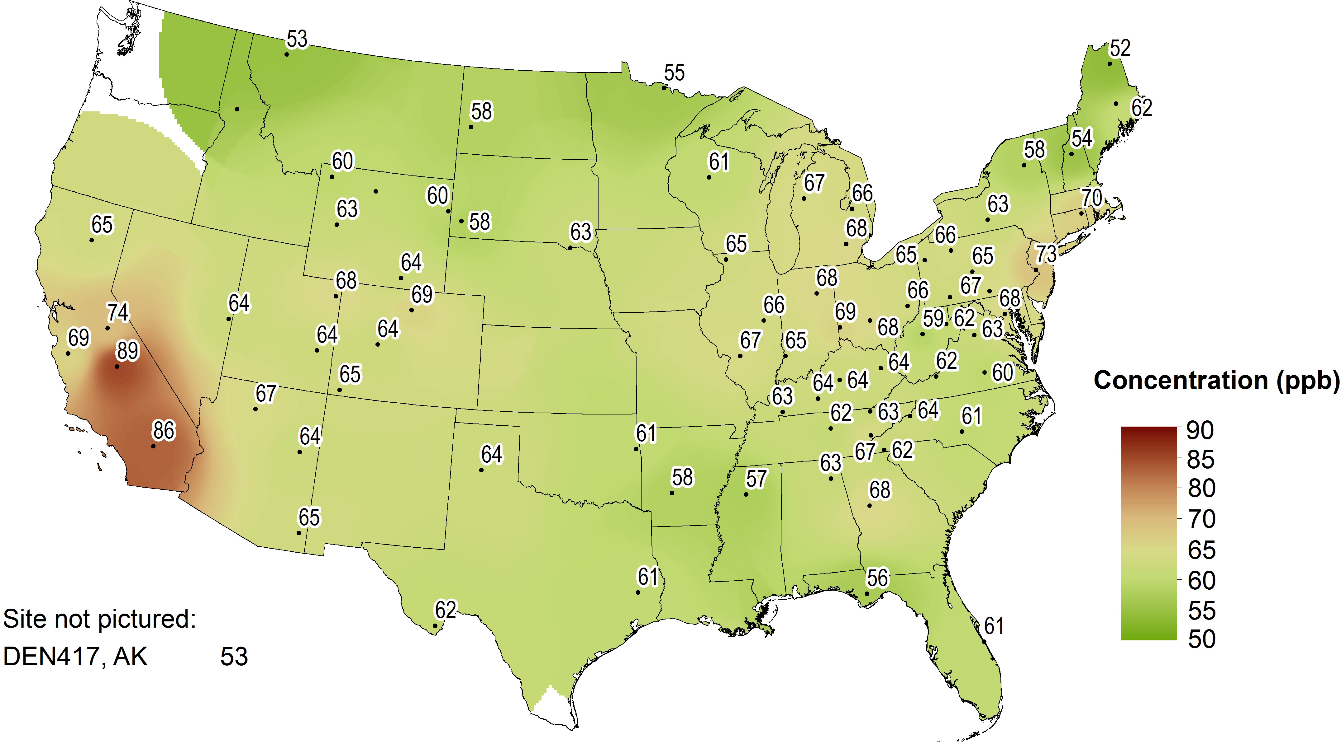
Eight-hour Ozone Concentrations
All CASTNET sites, with the exception of HOW191, ME; MCK231, KY; and ROM206, CO, are regulatory and may be used for NAAQS compliance. HOW191 does not meet regulatory siting criteria. MCK231 and ROM206 are co-located sites used solely for QA purposes and are designated as “NAAQS excluded.” Three-year averages of the fourth highest DM8A O3 concentrations for 2014 through 2016 are presented in Figure 2-1. Ozone concentrations were not included on the map if the 3-year average was not available because of incomplete data; these sites are shown as dots with no value. Three California CASTNET sites and one eastern site measured fourth highest DM8A O3 concentrations above the 2015 NAAQS. The highest 3-year design value of 89 parts per billion (ppb) was sampled at the Sequoia and Kings Canyon National Parks, CA (SEK430) site. The highest 3-year eastern concentration (73 ppb) was measured at Washington Crossing, NJ (WSP144). Table 2-1 lists sites with 2014–2016 O3 design values greater than 70 ppb.
Figure 2-1 Three-year Averages of Fourth Highest DM8A O3 Concentrations for 2014–2016
 Download Figure
Table 2-1 Sites with Design Values for 2014–2016 greater than 70 ppb
| Site ID | State | Sponsor | 3-year Average |
|---|---|---|---|
| SEK430 | California | NPS | 89 |
| JOT403 | California | NPS | 86 |
| YOS404 | California | NPS | 74 |
| WSP144 | New Jersey | EPA | 73 |
Figure 2-2 shows 2016 fourth highest DM8A O3 concentrations that met percent completeness criteria. During 2016, 10 eastern, 4 California sites, and 1 site in Utah measured fourth highest DM8A O3 concentrations greater than 70 ppb.
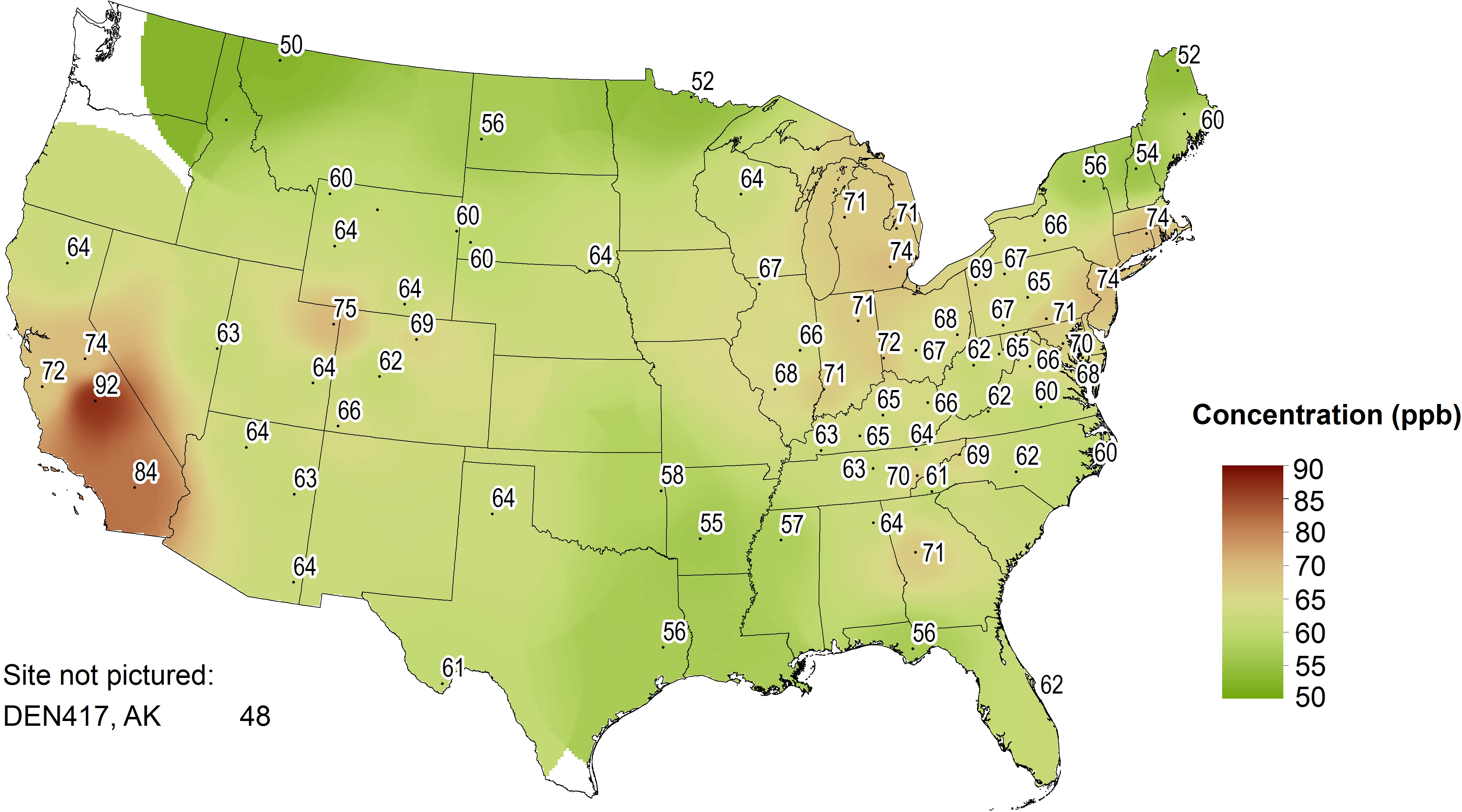
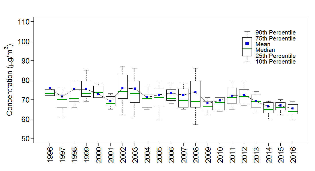
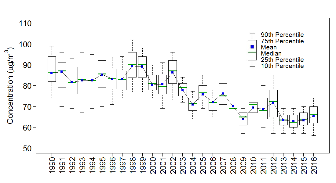
Figure 2-3 provides box plots depicting trends in 1-year mean, median, and annual distributions of fourth highest DM8A O3 concentrations from the eastern reference sites (right side) for 1990 through 2016 and for the western reference sites (left side) for 1996 through 2016. The reference sites were selected for their long-term data record and consistent performance. The eastern O3 data show an overall decline since 2002. The 2016 median data point, 64 ppb, was higher than the 2015 value of 63.5 ppb.
The western O3 data show an increase in fourth highest DM8A O3 concentrations from a 2009 minimum through 2012, followed by a decline through 2016. The 2016 median of the fourth highest DM8A O3 concentrations for the western reference sites was 66 ppb, the lowest value for the western reference sites.
Figure 2-3 Trends in Fourth Highest DM8A O3 Concentrations
Uinta Basin, Utah Ozone Concentrations
A network of O3 monitors throughout the Uinta Basin has measured elevated DM8A O3 levels. In fact, the Uinta Basin is one of only two places in the United States that measures wintertime O3 concentrations in excess of the NAAQS. Wyoming’s Upper Green River Basin is the other (CASTNET 2010 Annual Report; Wood, 2012).
The Uinta Basin is an enclosed basin that lies in the northeast corner of Utah and is part of a larger area known as the Colorado Plateau. The Basin is bounded on the north by the Uinta Mountain range, on the south by the Book and Roan Cliffs, on the west by the Wasatch Range, and on the east by elevated terrain separating it from the Piceance Basin in Colorado. The Green River runs through the Basin from northeast to southwest, exiting through the Book Cliffs via Desolation Canyon. The floor of the Basin is at approximately 1,463 meters above sea level with significant local surrounding topography with elevations of tens to hundreds of meters.
Wintertime air quality in the Uinta Basin deteriorates when strong inversion events persist over several days (Lyman et al., 2016). These multi-day inversions occur with stagnant, high-pressure weather conditions and sufficient snow cover to reflect incoming sunlight, which keeps the ground from absorbing sunlight and warming. Snow also provides energy for the chemical reactions that form O3 by increasing the amount of available solar radiation. Ozone forms in the atmosphere from reactions involving NOx and volatile organic compounds (VOC). Inversion conditions trap these pollutants near ground level and increase their concentrations and their subsequent ability to generate O3. Numerous exceedances of the NAAQS have occurred during winters with adequate snow cover and sustained high-pressure conditions, and no wintertime exceedances have ever been observed without snow cover. During lengthy inversion conditions, high O3 concentrations first form in the low- elevation center of the Basin. The O3 concentrations increase daily while expanding towards the Basin’s edges. The highest O3 concentrations occur primarily in areas at lowest elevation. Longer inversion episodes and episodes that occur late in the winter season tend to lead to higher O3 levels.
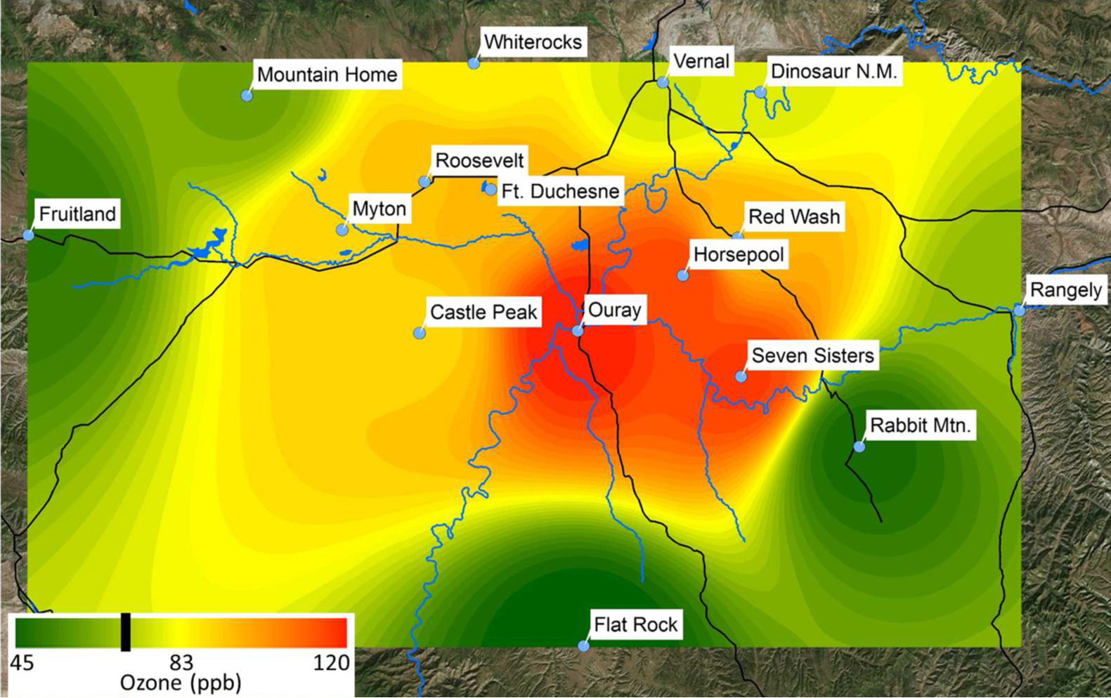
Figure 2-4 depicts DM8A O3 concentrations measured throughout the Basin on February 12, 2016. Color shading shows the magnitude of the O3 concentration (Lyman et al., 2016). Ozone monitoring locations are also shown. The site labeled Dinosaur N.M. is the DIN431 CASTNET site. Table 2-2 lists 8-hour average O3 concentrations measured in the Uinta Basin during the winter of 2015–2016. The highest DM8A O3 concentration exceeded 100 ppb
Figure 2-4 DM8A O3 Concentrations Measured throughout Uinta Basin on February 12, 2016
 Download Figure
Source:Lyman et al., 2016
Esri, DigitalGlobe, i-cubed, USDA, USGS, AEX, Getmapping, Aerogrid, IGN, IGP, swisstopo, and the GIS User Community
Note: Vertical black bar = 70 ppb
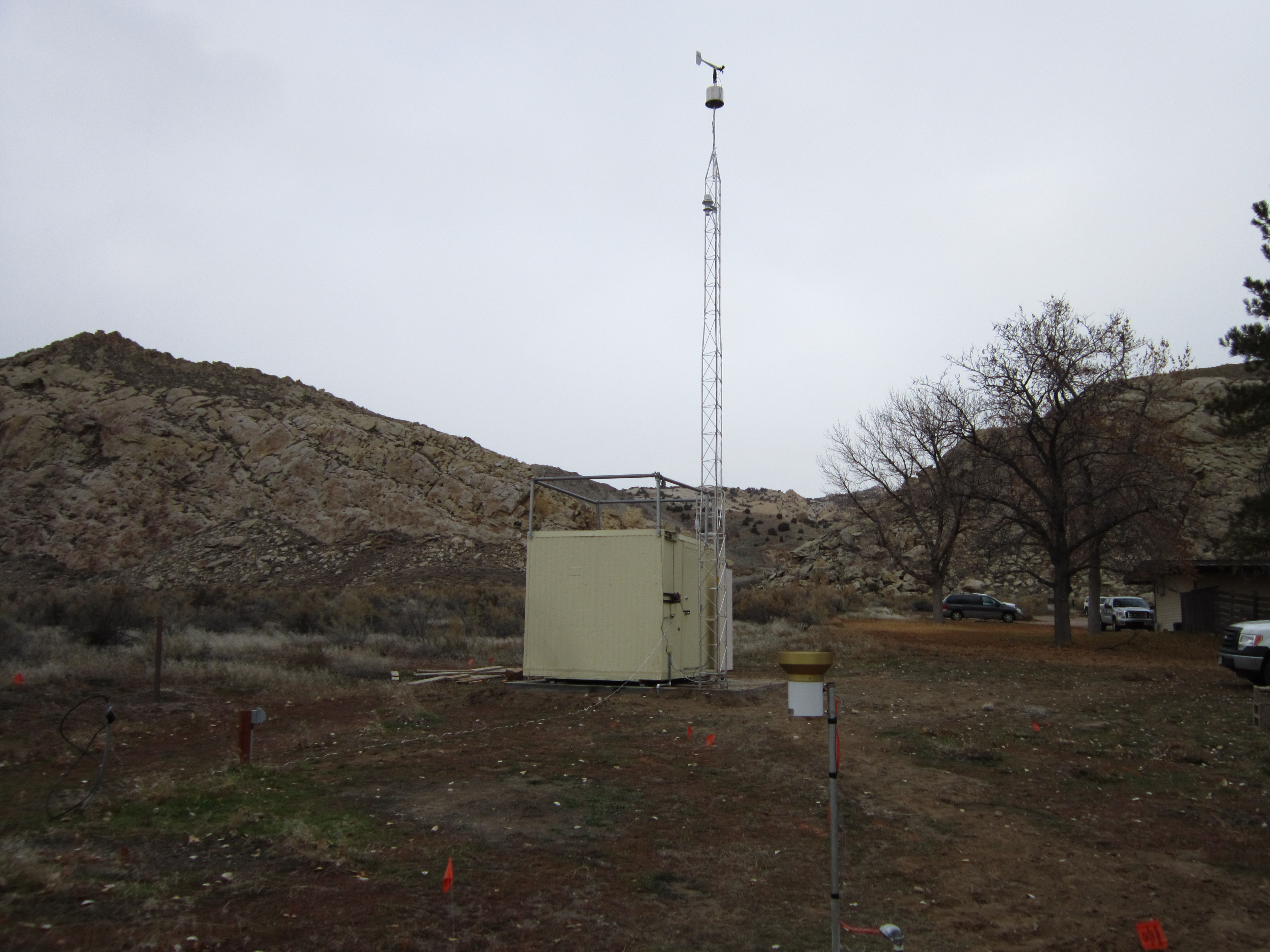
Air quality monitoring in the Basin began in 2006 when the Utah Department of Air Quality (UDAQ) installed monitors in Vernal to measure fine particulate matter (PM2.5), O3, and NOx. EPA added two monitoring sites in 2009, and the network further expanded to the number of sites shown in Figure 2-4 and Table 2-2. The NPS added the DIN431 CASTNET site in November 2013 (Appendix A). The site is located in the northeast corner of the Basin east of Vernal (Figure 2-4) at an elevation of 1,463 meters. Ozone concentrations measured at DIN431 were generally lower than those measured near the center of the Basin.
Table 2-2 8-hour Average O3 Concentrations Measured in the Uinta Basin during Winter 2015–2016
| Location | Site Elevation (Meters) |
Mean (ppb) | Maximum (ppb) | Minimum (ppb) | Fourth Highest DM8A (ppb) |
Number of Exceedances |
|---|---|---|---|---|---|---|
| Dinosaur NM | 1463 | 37.0 | 83.6 | 9.5 | 75.3 | 5 |
| Ouray | 1464 | 37.7 | 120.6 | 8.8 | 96.8 | 11 |
| Fort Duchesne | 1559 | 31.9 | 96.8 | 6.8 | 90.4 | 9 |
| Horsepool | 1569 | 44.1 | 115.8 | 16.4 | 93.6 | 11 |
| Roosevelt | 1587 | 35.2 | 96.0 | 10.8 | 84.8 | 10 |
| Castle Peak | 1605 | 39.0 | 99.8 | 16.3 | 84.0 | 8 |
| Vernal | 1606 | 34.7 | 78.4 | 10.3 | 73.6 | 5 |
| Myton | 1610 | 38.7 | 95.1 | 16.6 | 85.5 | 8 |
| Seven Sisters | 1618 | 39.3 | 117.5 | 11.0 | 100.9 | 9 |
| Rangely | 1648 | 36.9 | 67.4 | 19.8 | 59.8 | 0 |
| Red Wash | 1689 | 39.9 | 96.0 | 18.6 | 83.5 | 7 |
| Rabbit Mountain | 1879 | 32.9 | 52.9 | 11.8 | 48.2 | 0 |
| Whiterocks | 1893 | 43.4 | 86.1 | 25.3 | 81.3 | 7 |
| Fruitland | 2021 | 36.4 | 62.4 | 9.3 | 53.1 | 0 |
| Mountain Home | 2234 | 46.7 | 72.4 | 32.6 | 64.3 | 1 |
| Flat Rock | 2274 | 44.2 | 58.2 | 30.0 | 54.6 | 0 |
Source:Lyman et al., 2016
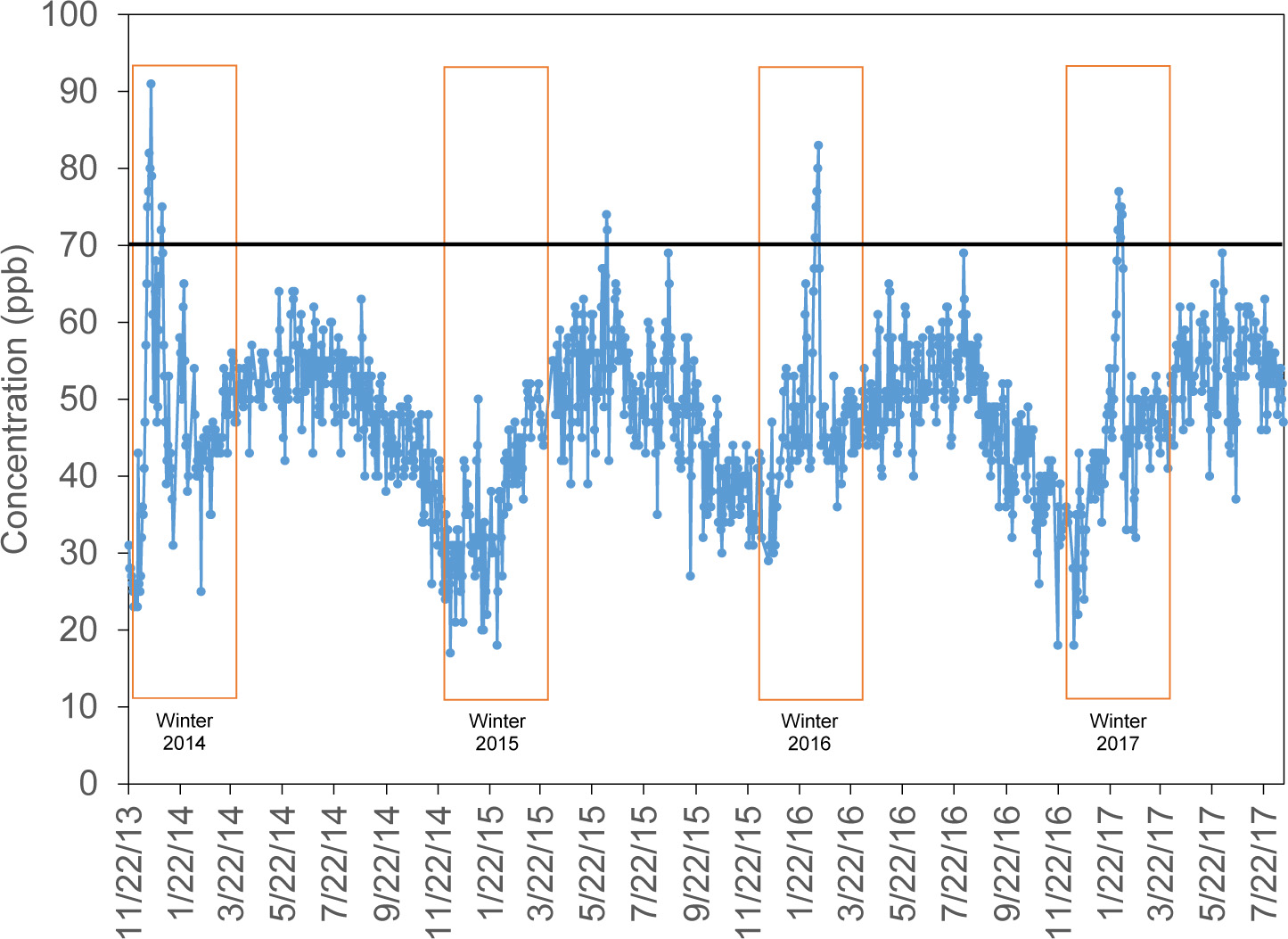
Figure 2-5 presents a time series of DM8A O3 concentrations measured at DIN431 from its inception through mid-2017. Several DM8A O3 concentrations exceeded 70 ppb. Most of the high concentrations were observed during first quarter. However, several high values were measured during summer months. Some investigators (Ute Indian Tribe, 2016) have concluded that stratospheric O3 intrusions and wildfires contribute to elevated spring and summer O3 levels. No concentrations greater than 70 ppb were sampled during the first quarter of 2015 because of a lack of snow cover (Neeman et al., 2015).
Figure 2-5 Time Series of DM8A O3 Concentrations Measured at DIN431 from November 2013 through July 2017
 Download Figure
Dinosaur National Monument (DIN431), North (full site)
Table 2-3 summarizes the 10 highest DM8A O3 concentrations annually at DIN431 over the four years 2014 through 2017.
Table 2-3 Ten Highest DM8A O3 Concentrations at DIN431 for 2014 through 2017
| Date | DM8A (ppb) | Rank |
|---|---|---|
| 2014 | ||
| 1/1/2014 | 69 | 1 |
| 1/26/2014 | 65 | 2 |
| 5/18/2014 | 64 | 3 |
| 6/3/2014 | 64 | 3 |
| 6/5/2014 | 64 | 3 |
| 6/4/2014 | 63 | 6 |
| 8/23/2014 | 63 | 6 |
| 1/25/2014 | 62 | 8 |
| 6/28/2014 | 62 | 8 |
| 6/1/2014 | 61 | 10 |
| 6/2/2014 | 61 | 10 |
| 6/13/2014 | 61 | 10 |
| 2015 | ||
| 6/8/2015 | 74 | 1 |
| 6/9/2015 | 72 | 2 |
| 8/20/2015 | 69 | 3 |
| 6/3/2015 | 67 | 4 |
| 6/4/2015 | 67 | 4 |
| 6/7/2015 | 66 | 6 |
| 6/19/2015 | 65 | 7 |
| 8/21/2015 | 65 | 7 |
| 6/20/2015 | 64 | 9 |
| 5/12/2015 | 63 | 10 |
| 6/18/2015 | 63 | 10 |
| 2016 | ||
| 2/13/2016 | 83 | 1 |
| 2/12/2016 | 80 | 2 |
| 2/11/2016 | 77 | 3 |
| 2/10/2016 | 75 | 4 |
| 2/9/2016 | 71 | 5 |
| 8/2/2016 | 69 | 6 |
| 2/8/2016 | 67 | 7 |
| 2/14/2016 | 67 | 7 |
| 1/29/2016 | 65 | 9 |
| 5/6/2016 | 65 | 9 |
| 2017 | ||
| 2/1/2017 | 77 | 1 |
| 2/2/2017 | 75 | 2 |
| 2/4/2017 | 75 | 2 |
| 2/5/2017 | 74 | 4 |
| 1/31/2017 | 72 | 5 |
| 2/3/2017 | 71 | 6 |
| 6/3/2017 | 69 | 7 |
| 1/30/2017 | 68 | 8 |
| 2/6/2017 | 67 | 9 |
| 9/7/2017 | 66 | 10 |
| 3-year Averages | ||
| Date | DM8A (ppb) | |
| 2014–2016 | 68 | |
| 2015–2017 | 72 | |
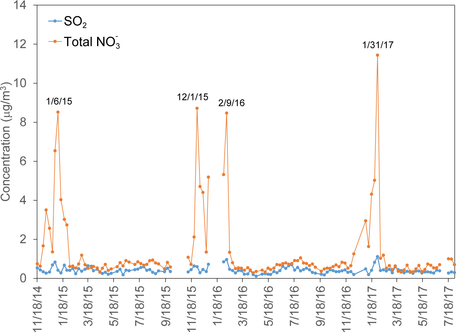
Data from DIN431 also provides information on SO2 and total NO3- concentrations in micrograms per cubic meter (μg/m 3 ) of air over the period November 2014 through July 2017. Figure 2-6 presents weekly average concentrations. Sulfur dioxide concentrations were low throughout the period while total NO3- concentrations showed occasional spikes that were 5 to 10 times higher than average. Two periods with high DM8A O3 concentrations (Table 2-3) were observed during weeks with high total NO3- concentrations.
Chapter 3: Nitrogen Pollutant Concentrations
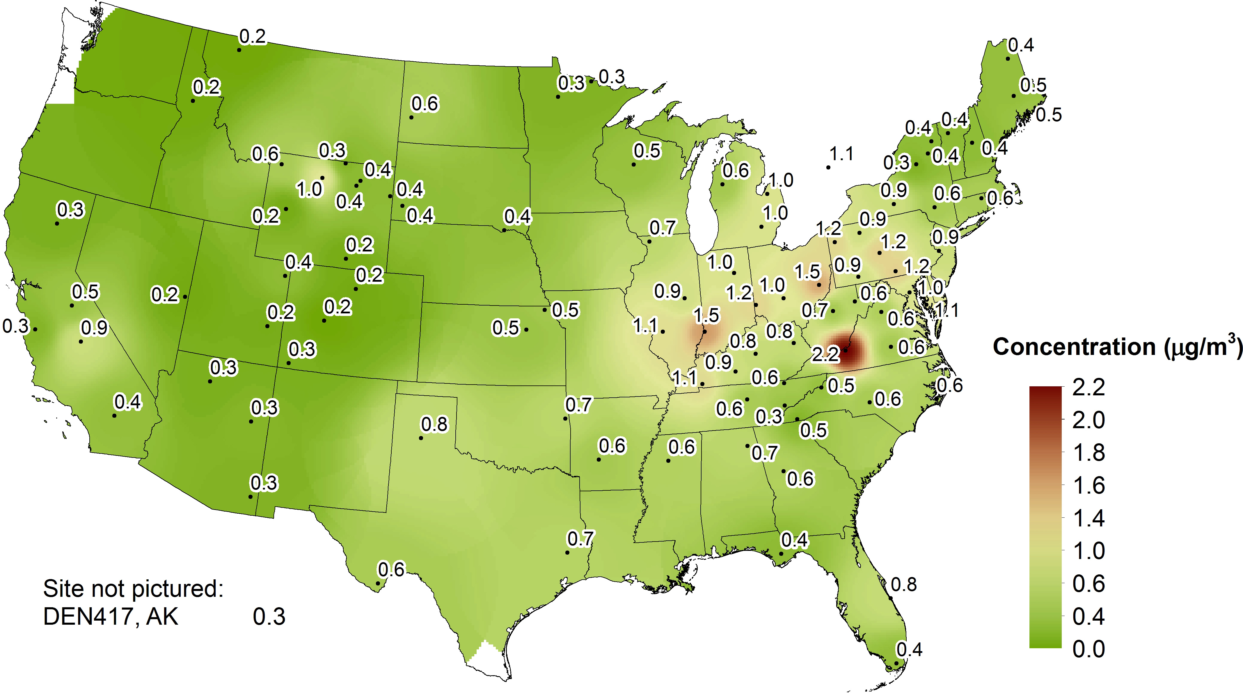
During 2016, weekly average concentrations of nitric acid, particulate nitrate, and particulate ammonium were measured using 3-stage filter packs at 95 CASTNET monitoring stations. Maps of 2016 annual mean total nitrate (nitric acid plus nitrate) and ammonium concentrations show the geographic distribution of the two pollutants measured. Box plots provide trends in annual mean total nitrate and ammonium concentrations aggregated over 34 eastern and 16 western reference sites. The nitrogen pollutants measured at the 34 eastern reference sites declined over the 27-year period from 1990 through 2016. Annual mean concentrations of total nitrate were reduced by 48 percent from 1990 through 2016. Ammonium concentrations declined by 63 percent. Total nitrate and ammonium concentrations measured at the 16 western reference sites were reduced by 34 percent and 31 percent, respectively, over the 21-year period 1996 through 2016.
Annual mean concentrations of total NO3- (HNO3 + NO3-) and NH4+ for 2016 are presented in two maps in this chapter. Additional maps of 2016 quarterly mean concentrations are provided in CASTNET quarterly data reports (Wood, 2016a; 2016b; 2017a; 2017b). Trends in annual mean concentrations over the 27-year period, 1990 through 2016, were calculated from measurements from the 34 CASTNET eastern reference sites and for the 21-year period, 1996 through 2016, from data measured at the 16 CASTNET western reference sites. See Appendix A for the designated reference sites.
Total Nitrate Concentrations
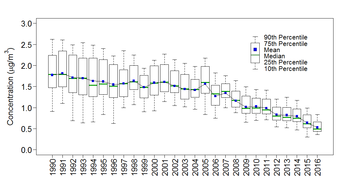
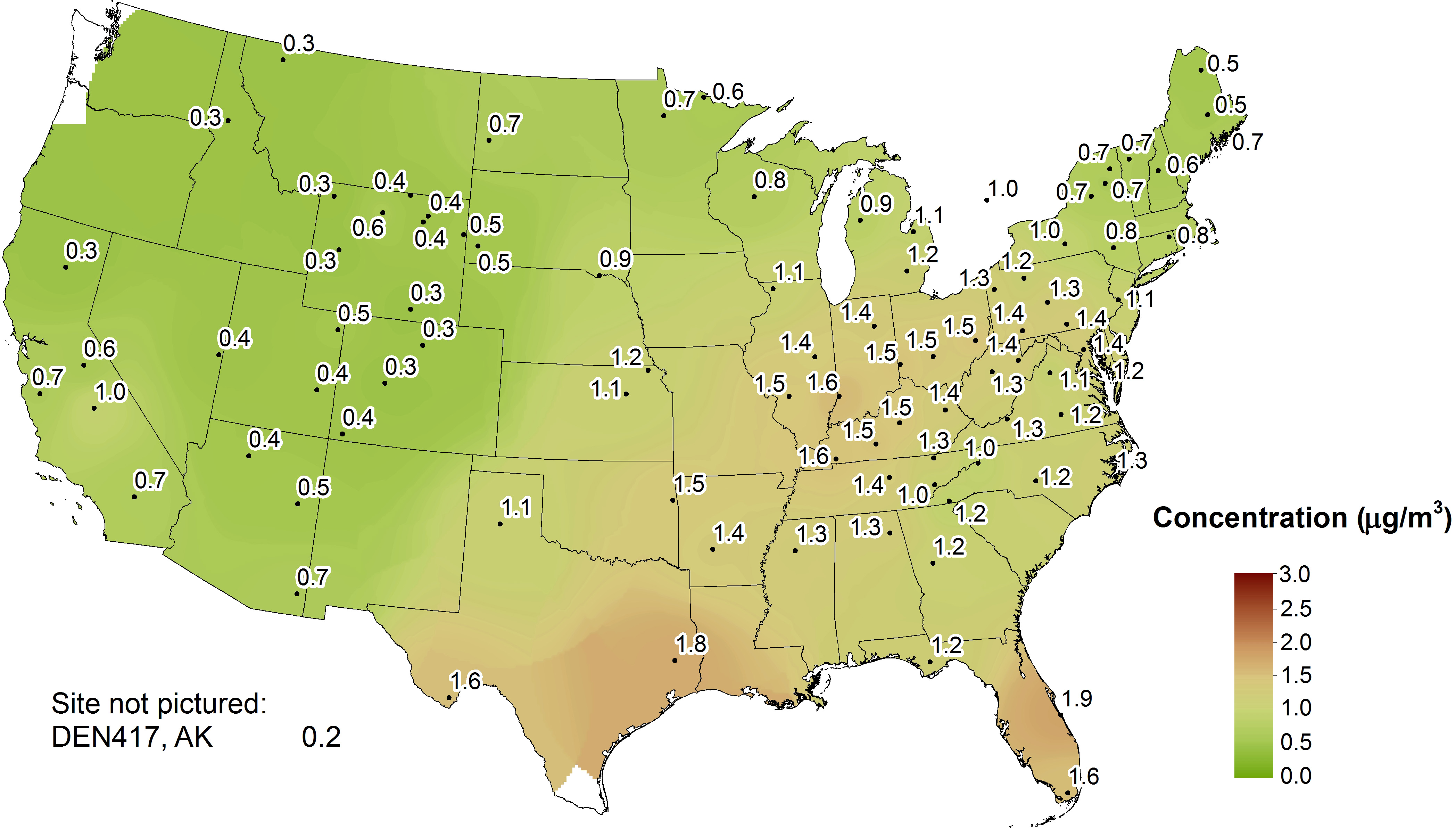
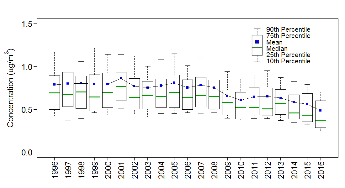
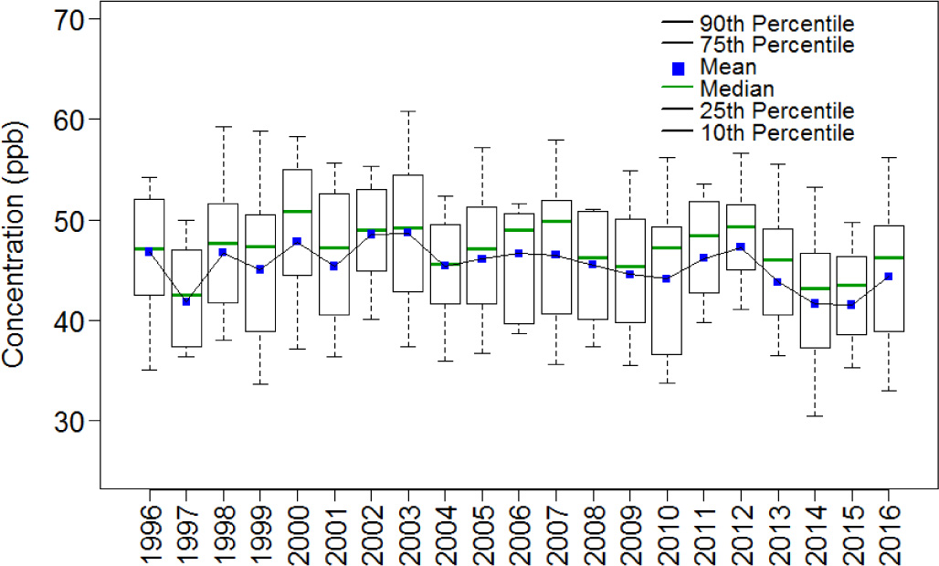
Mean total NO3- concentrations measured in 2016 are presented in the map in Figure 3-1. To illustrate trends, Figure 3-2 provides box plots of total NO3- levels for the eastern and western reference sites through 2016. Each box presents the mean and median concentrations and the 10th, 25th, 75th, and 90th percentiles for that year. The data shown on the right side of the figure were aggregated from the 34 eastern reference sites. The data show no trend in mean concentrations until 2000 when total NO3- levels began to decline in response to NOx emission controls. Total NO3- levels measured at the eastern reference sites were reduced by 53 percent from a mean value of 3.1 μg/m 3 in 2000 to a mean value of 1.5 μg/m 3 in 2016. Over the history of the network, 3-year mean levels declined from 3.0 μg/m 3 for 1990–1992 to 1.6 μg/m 3 for 2014–2016, producing a 48 percent reduction in total NO3-.
The left side of Figure 3-2 shows data aggregated from the 16 western sites. Total NO3- levels declined from 1.1 μg/m 3 to 0.6 μg/m 3 from 2000 through 2016, a 43 percent reduction. The 3-year mean total NO3- concentration for 2014–2016 was 34 percent lower than the corresponding 1996– 1998 level. The 3-year mean concentration was 1.0 μg/m 3 for 1996–1998 and 0.7 μg/m 3 for 2014–2016.
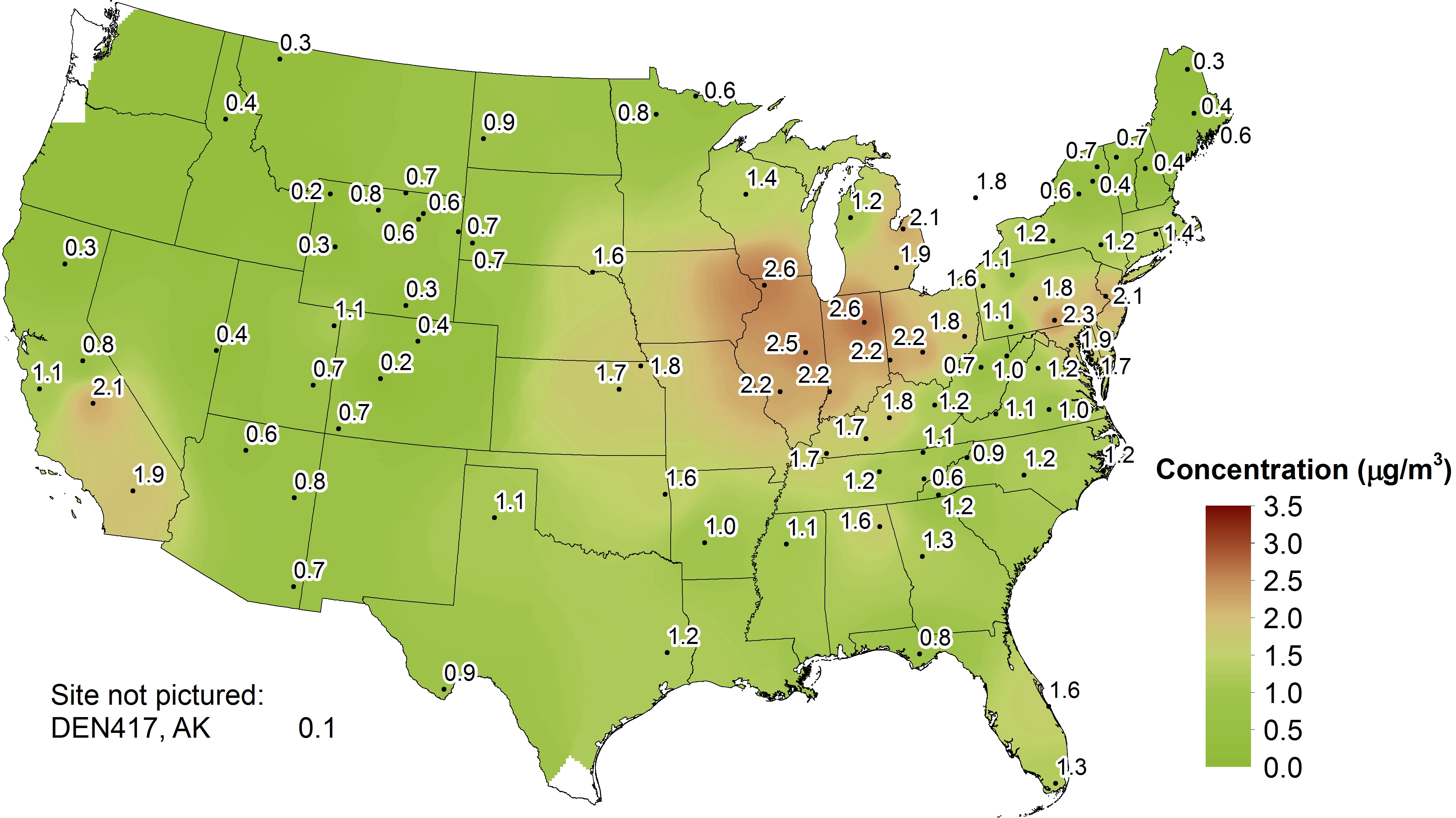
Figure 3-2 Trends in Annual Mean Total NO3- Concentrations
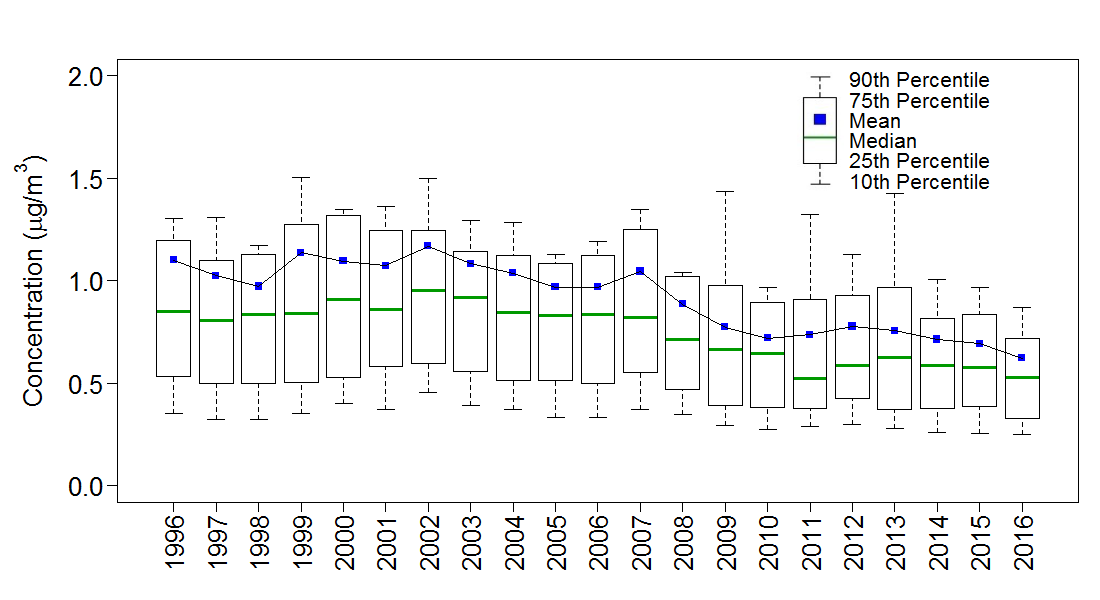
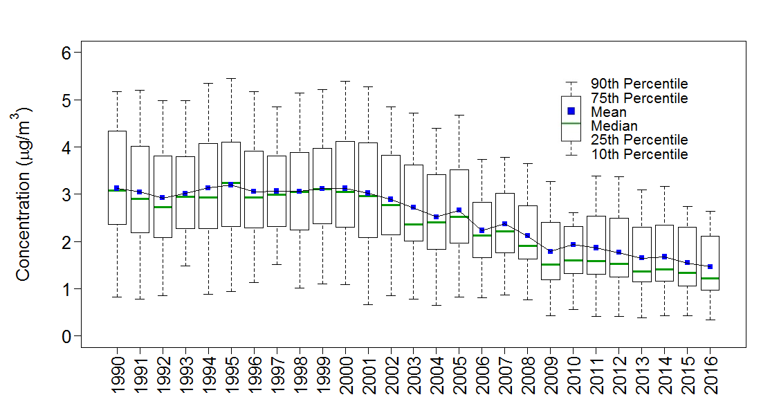
Figure 3-3 illustrates the trend in NOx emissions from regulated EGUs operating in the eastern United States from 1990 through 2016. The 27-year decline in aggregated EGU emissions was 86 percent.
Figure 3-3 Trend in Annual Composite NOx Emissions from Regulated EGUs Operating in the Eastern United States
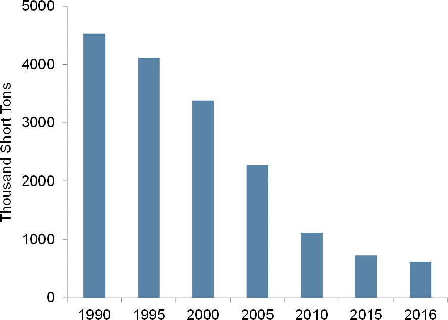
Source: EPA (2017)
Download FigureParticulate Ammonium Concentrations
A map of 2016 mean particulate NH4+ concentrations is provided in Figure 3-4. Figure 3-5 shows box plots of NH4+ concentrations. The trend diagram for the eastern sites (right side) shows a reduction in mean NH4+ levels from 1990–1992 to 2014–2016. The 1990–1992 mean concentration was 1.8 μg/m 3 , and the 2014–2016 value was 0.7 μg/m 3 , a 63 percent decline. Similar to total NO3-, the eastern NH4+ concentrations began to decline in 2000 and have been reduced from 1.6 μg/m 3 in 2000 to 0.5 μg/m 3 in 2016. The western reference sites show a decline from 0.3 μg/m 3 in 1996–1998 to 0.2 μg/m 3 in 2014–2016, a 31 percent reduction.
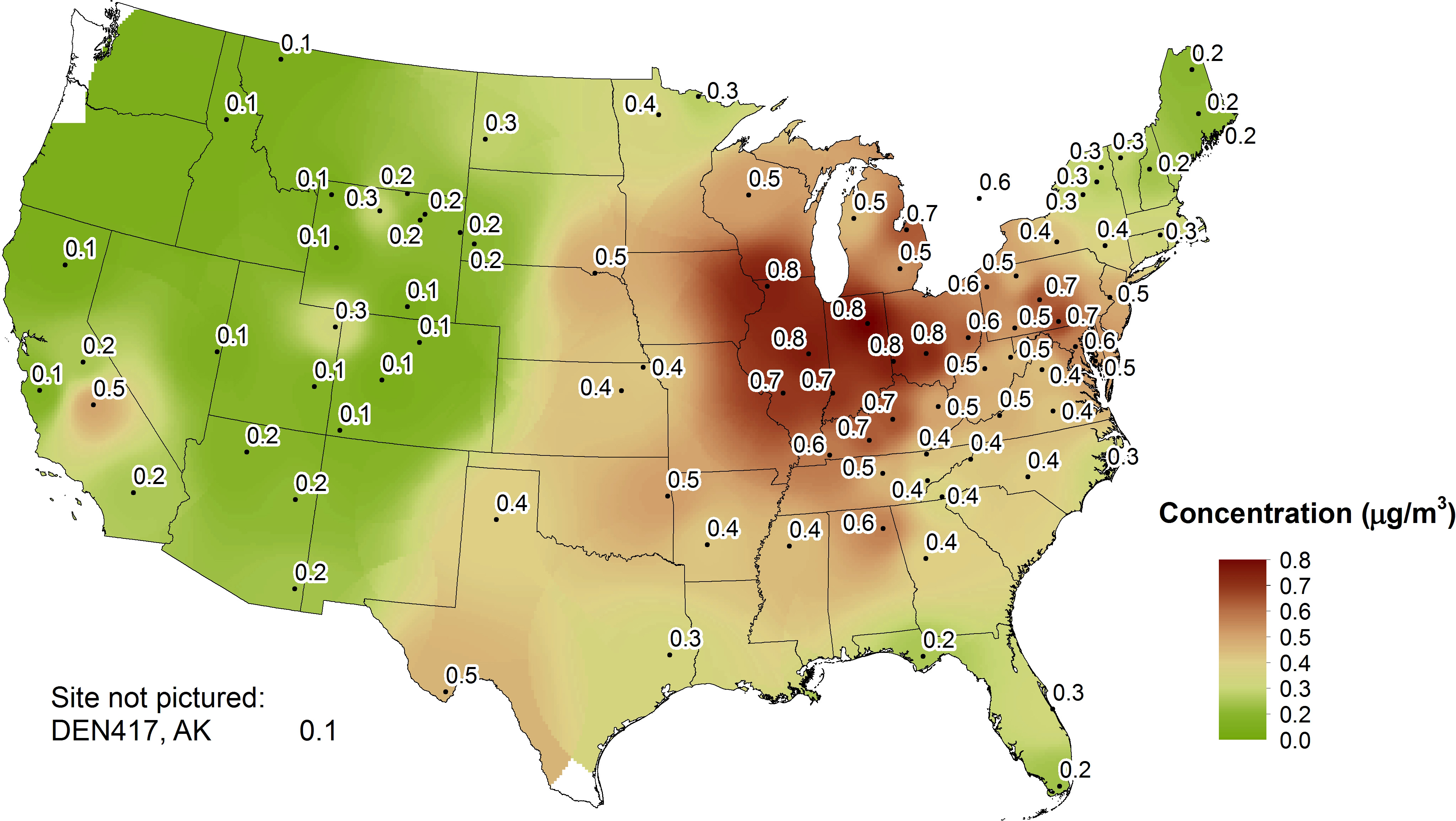
Figure 3-5 Trends in Annual Mean NH4+ Concentrations
Quality Assurance Program Results
Precision of Filter Pack Measurements
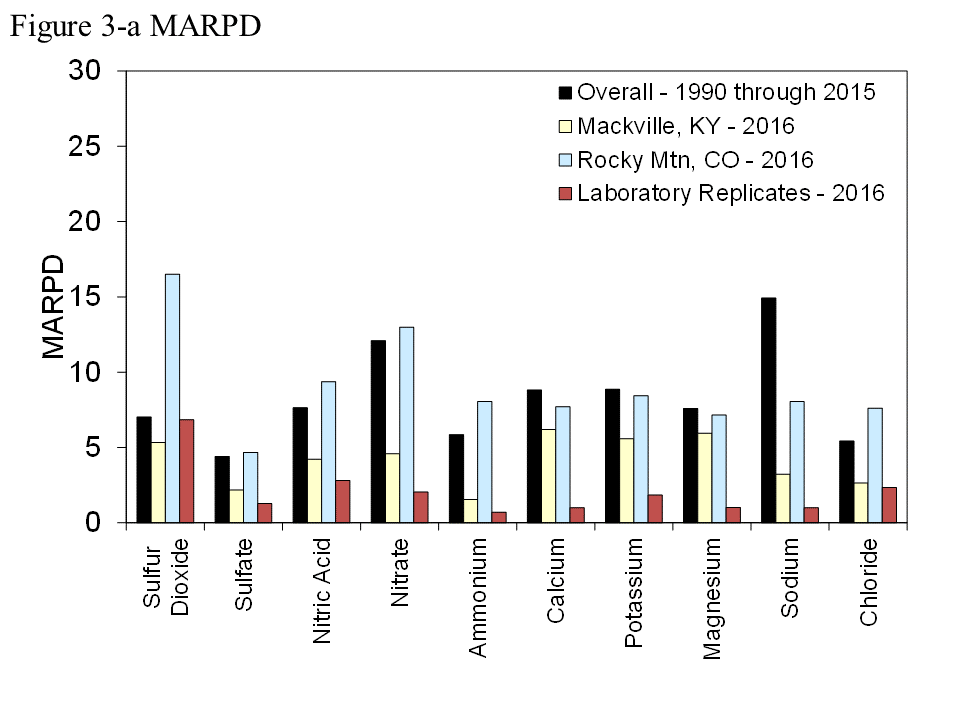
Historical (1990 through 2015) mean absolute relative percent difference (MARPD) data for all 11 co-located site pairs operated over the history of the network are provided in the bar chart in Figure 3-a. The 2016 data for the current co-located sites at MCK131/231 and ROM406/206 are also provided. The precision criterion is a MARPD of 20 percent. Historical and 2016 measurements met the criterion for each analyte. The MARPD for SO2 at ROM406/206 was unusually high because of the imprecision of lower concentrations measured during the first two quarters.
Figure 3-a Historical and 2016 Precision Results for Atmospheric Concentrations and Laboratory Replicate Samples
 Download Figure
The 2016 analytical precision results for 10 analytes are also presented in Figure 3-a. The results were based on analysis of 5 percent of the samples that were randomly selected for replication in each batch. The results of in-run replicate analyses were compared with the original concentration results. The laboratory precision data met the 20 percent measurement criterion.
Data Completeness
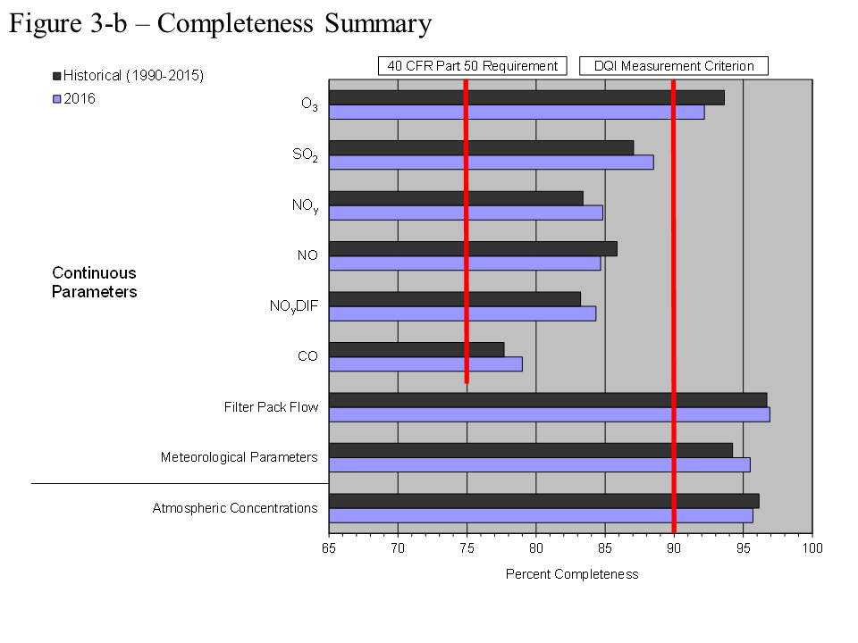
Completeness is defined as the percentage of valid data points obtained from a measurement system relative to total possible data points. The CASTNET measurement criterion for completeness requires a minimum completeness of 90 percent for every parameter for each quarter. The historical results and the results for 2016 are given in Figure 3-b. Historical results for trace-level gas measurements represent data from 2013–2015. The completeness criterion was met for atmospheric (filter pack) and O3 concentrations, filter pack flow, and meteorological measurements. Completeness of trace-level gas measurements (Chapter 6) met the completeness requirements of 40 CFR Part 50 (EPA, 2015c).
Figure 3-b Historical and 2016 Percent Completeness of Measurements (black bars are 1990–2015 for long-term data and 2013–2015 for trace-level gas data)
 Download Figure
Update on the Ammonia Monitoring Network
The Ammonia Monitoring Network (AMoN) operates passive ammonia samplers at 103 locations, 69 of which are located at CASTNET sites. AMoN is managed by the National Atmospheric Deposition Program. The network has been in operation since 2007 and provides information on 2-week integrated ammonia concentrations. Like other NADP networks, the goal of AMoN is to operate a long-term (i.e., for several decades), spatially diverse network with consistent measurements, covering all sensitive ecoregions of the continental United States.
Reduced nitrogen [ammonia (NH3) + NH4+] is an important component to total nitrogen deposition. Wet deposition of NH4+ measured by NTN has been increasing in many areas of the United States over the past 10 years; however, until 2007, gaseous NH3 concentrations were not routinely measured. Ammonia is the most prevalent alkaline gas in the atmosphere and is released into the air from a variety of agricultural sources (animal waste, fertilizer application, and agricultural burning), biological sources, gas and oil production and processing, and combustion. Agriculture is by far the largest source, producing approximately 80 percent of gaseous NH3 emissions (EPA National Emissions Inventory, 2014). Although NH3 is beneficial when used as NH3-based fertilizer, it can have a negative effect on the environment when it reacts with acidic ions such as SO42- and NO3- to form PM2.5, which contributes to negative impacts on human health and visibility degradation. Atmospheric deposition of reduced nitrogen also contributes to eutrophication of sensitive ecosystems, decreases in species diversity, and increases in invasive species.
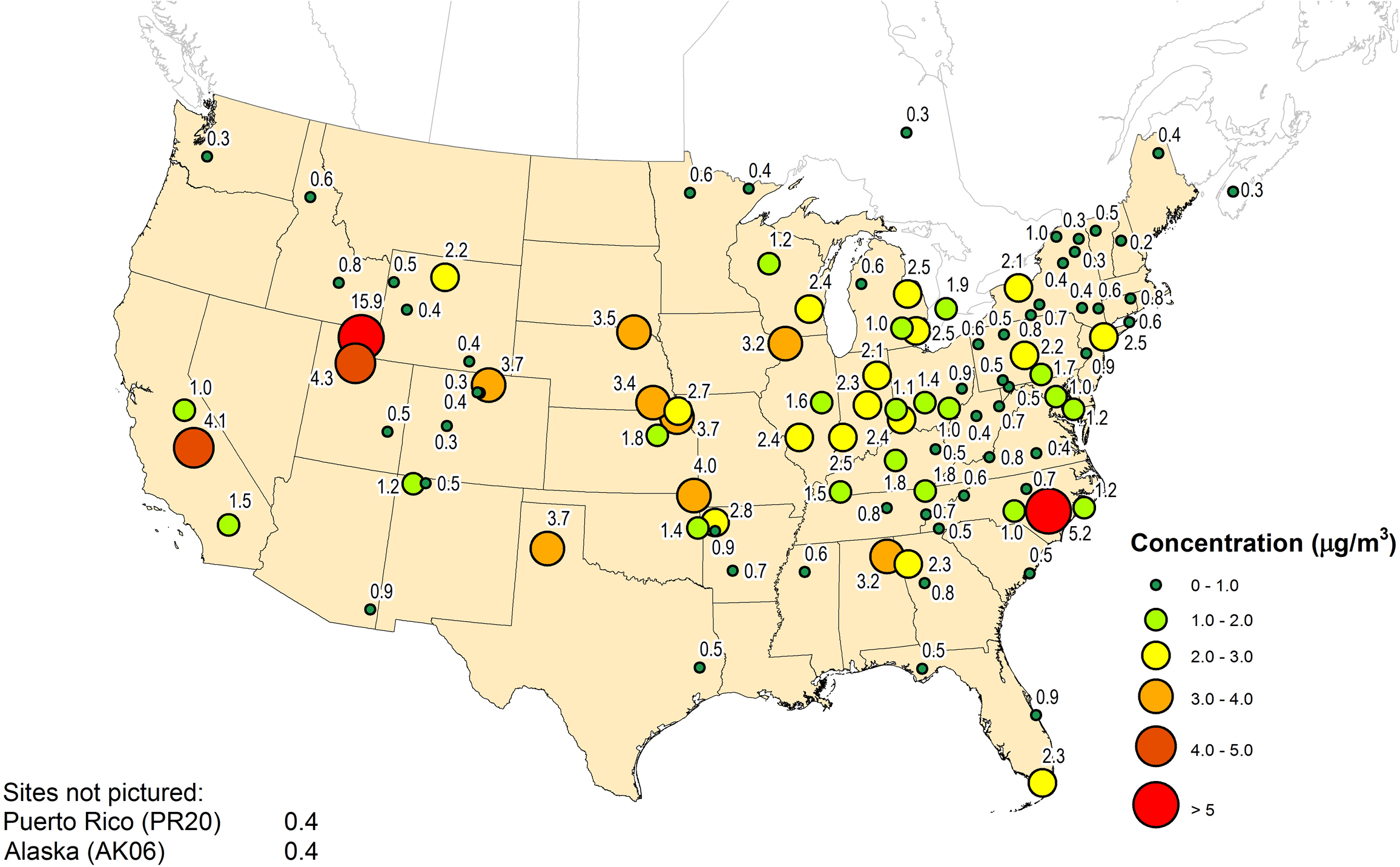
Average annual NH3 concentrations for 2016 for the sites that met completeness requirements are mapped in Figure 4-1 and show a wide range of concentrations from a low of 0.2 μg/m 3 in New Hampshire (NH02) to a high of 15.9 μg/m 3 in northern Utah (UT01). The Utah monitoring site is located on a Utah State University research farm and small quantities of livestock are often present (Martin and Baasandorj, 2016). The farm is situated in the Cache Valley, an area with frequent stagnant weather. The next highest concentrations ranged from 3.4 to 4.3 μg/m 3 at eight sites west of the Mississippi River. The highest concentration east of the Mississippi was observed at Cranberry, NC (NC02) with a measured concentration of 5.2 μg/m 3 . High NH3 concentrations can be attributed to local emissions from hog and cattle feeding and waste and crop fertilization and production.
Chapter 5: Sulfur Pollutant Concentrations
During 2016, weekly average concentrations of sulfur dioxide and particulate sulfate were measured using 3-stage filter packs at 95 CASTNET monitoring stations. Maps of 2016 annual mean concentrations show the geographic distribution of the two pollutants across the United States. Annual sulfur dioxide and sulfate concentrations were aggregated over 34 eastern and 16 western reference sites in order to estimate trends, which are depicted using box plots. The sulfur dioxide pollutants measured at the eastern reference sites declined by 86 percent over the 27-year period from 1990 through 2016. Particulate sulfate concentrations were reduced by 70 percent. Measured concentrations of sulfur dioxide and sulfate have decreased steadily since 2005. Sulfur dioxide and sulfate concentrations measured at the 16 western reference sites have decreased by 46 and 31 percent, respectively, over the 21-year period 1996 through 2016.
Annual mean concentrations of SO2 and SO42- for 2016 are presented in this chapter. Additional maps of 2016 quarterly mean concentrations are provided in CASTNET quarterly data reports (Wood, 2016a; 2016b; 2017a; 2017b). Trends in annual mean concentrations over the 27-year period, 1990 through 2016, were derived from measurements from the 34 CASTNET eastern reference sites and for the 21-year period, 1996 through 2016, from data measured at the 16 CASTNET western reference sites. See Appendix A for descriptions of the designated reference sites.
Sulfur Dioxide Concentrations
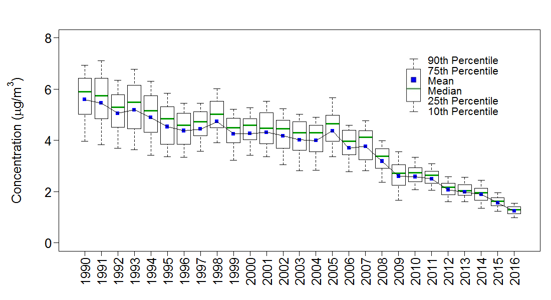
Annual mean SO2 concentrations are shown in Figure 5-1 for 2016. Annual mean concentrations were highest in the Midwest and East near and downwind of the Ohio River. Box plots of annual mean SO2 concentrations aggregated over the 34 eastern reference sites from 1990 through 2016 (right side) and the 16 western reference sites from 1996 through 2016 (left side) are depicted in Figure 5-2. The y-axes on the western and eastern plots have different scales because concentrations measured at the western CASTNET sites were much lower than those measured at the eastern sites. Three-year mean concentrations for the CASTNET eastern reference sites for 1990–1992 and 2014–2016 were 8.8 μg/m 3 and 1.2 μg/m 3 , respectively. This change constitutes an 86 percent reduction in 3-year mean SO2 concentrations between the two periods. The 2016 mean level of 0.8 μg/m 3 was the lowest concentration measured by the eastern reference sites in the history of the network and represents a significant decline from the 2005 mean concentration of 6.0 μg/m 3 .
The box plots for the western reference sites indicate a decline in annual mean SO2 concentrations aggregated over the 16 sites. Three-year mean SO2 concentrations for 1996–1998 and 2014–2016 were 0.6 μg/m 3 and 0.3 μg/m 3 , respectively. This change constitutes a 46 percent reduction in 3-year mean SO2 concentrations at the CASTNET western reference sites over the 21 years.
The 2016 average sulfur dioxide concentration for the eastern reference sites was 0.8 µg/m 3 . The eastern sulfur dioxide data show a substantive decline since 1997. The reduction (86 percent) in sulfur dioxide concentrations over the period 1990 through 2016 is consistent with the reduction (94 percent) in sulfur dioxide emissions from EGUs operating in the eastern United States.
Figure 5-2 Trends in Annual Mean SO2 Concentrations
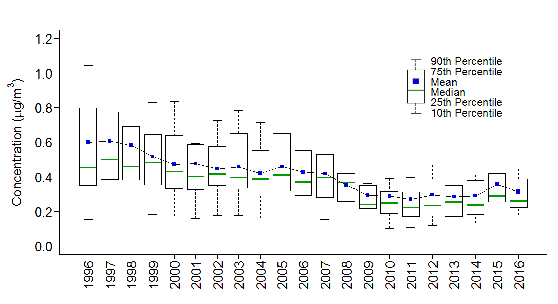
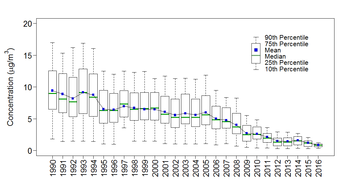
Figure 5-3 Trend in Annual Composite SO2 Emissions from Regulated EGUs Operating in the Eastern United States
 Download Figure
Figure 5-3 illustrates the trend in SO2 emissions from regulated EGUs from 1990 through 2016 aggregated over the eastern United States. The 27-year decline in aggregated emissions was 94 percent, which is consistent with the 86 percent reduction (Figure 5-2) in annual mean SO2 concentrations aggregated over the CASTNET eastern reference sites.
Particulate Sulfate Concentrations
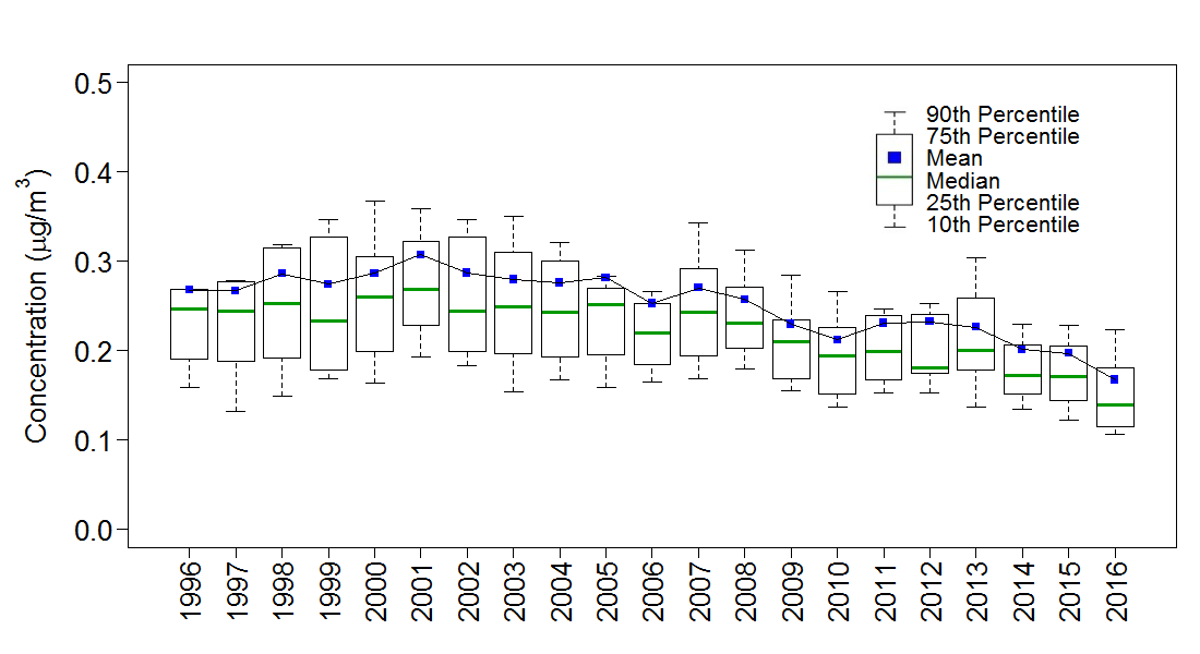
Figure 5-4 shows a map of 2016 annual mean particulate SO42- concentrations. Figure 5-5 provides box plots of annual mean SO42- concentrations from the 34 eastern reference sites (right side) and 16 western reference sites. The figure shows a substantial decline in SO42- over the 27 years for the eastern CASTNET reference sites. Of particular interest, concentrations declined rapidly from 2005 through 2016. The difference between 3-year means from 1990–1992 to 2014–2016 depicts a 70 percent reduction in SO42- from 5.4 μg/m 3 to 1.6 μg/m 3 . The 2016 mean SO42- level of 1.2 μg/m 3 for the eastern reference sites was the lowest in the history of the network. The box plots for the western reference sites are provided on the left side of Figure 5-5. The data show a 31 percent reduction in annual mean SO42- concentrations aggregated over the 16 sites with 1996–1998 and 2014–2016 concentrations of 0.8 μg/m 3 and 0.5 μg/m 3 , respectively.
The 2016 average sulfate concentration for the eastern reference sites was 1.2 µg/m 3 , the lowest level in the history of the network. The eastern sulfate data show a substantive decline since 2005. Sulfate concentrations declined more slowly than sulfur dioxide concentrations at the eastern reference sites. Western sulfate concentrations were lower and decreased at a slower rate than concentrations measured at the eastern sites.
Figure 5-5 Trends in Annual Mean SO42- Concentrations
Chapter 6: Continuous Trace-level Gas Concentrations
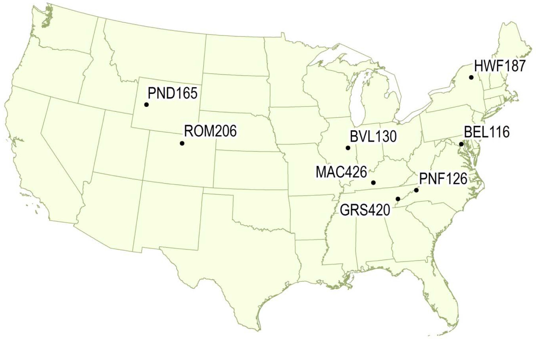
Trace-level, gaseous, air quality monitors were operated continuously at eight CASTNET sites during 2016. EPA operated six monitors and NPS operated two. The measurements at these sites were performed to (1) provide data for regional model input and evaluation, (2) generate data to elucidate atmospheric processes such as ozone and fine particulate matter formation, and (3) support EPA NCore monitoring. Total reactive oxides of nitrogen were measured at all eight sites, sulfur dioxide at four sites, and carbon monoxide at two sites. Total reactive oxides of nitrogen concentrations were highest at the suburban Beltsville, MD site and lowest at the high-elevation, mountainous sites.
Trace-level gas analyzers were deployed at six EPA and two NPS CASTNET sites during 2016. Other federal, tribal, and state agencies also measured NO/NOy at CASTNET or nearby sites in Maine, North Dakota, Oklahoma, and South Dakota. Table 6-1 lists the site locations, start dates, and the trace-level gas parameters measured at each CASTNET site. These data were sampled continuously and archived as 1-hour values.
| Site Location | Start Dates | Measurements |
|---|---|---|
| Beltsville, MD (BEL116) | March 2005 | NO/NOy and SO2 |
| Mammoth Cave National Park, KY (MAC426)* | May 2009 | NO/NOy, SO2, and CO |
| Bondville, IL (BVL130) | July 2012 | NO/NOy, SO2, and CO |
| Huntington Wildlife Forest, NY (HWF187) | November 2012 | NO/NOy |
| Pinedale, WY (PND165) | May 2013 | NO/NOy |
| Cranberry, NC (PNF126) | October 2013 | NO/NOy |
| Rocky Mountain National Park, CO (ROM206) | October 2013 | NO/NOy |
| Great Smoky Mountains National Park (GRS420)* | November 2014 | NO/NOy and SO2 |
Note: *Operated by NPS
NOy is defined as NOx [NO + nitrogen dioxide (NO2)] plus NOz [HNO3, nitrous acid (HONO), peroxyacetyl nitrate, peroxyproyl nitrate, other organic nitrates, and nitrite]. It consists of reactive gases that are considered precursors of O3 and PM2.5. Measurement of NOy begins with conversion to NO using a thermal catalytic converter and measurement of the NO by chemiluminescence. Continuous SO2 is measured using ultraviolet fluorescence, and CO is measured by gas filter correlation.
Figure 6-1 provides a map of the CASTNET continuous trace-level gas monitoring locations. All EPA sites were operated according to the CASTNET QAPP Appendix 11, “Procuring, Installing, and Operating NCore Air Monitoring Equipment at CASTNET Sites” (Wood, 2015). NPS sites were operated according to the NPS QAPP (Air Resource Specialists, 2015).
Figures 6-2 through 6-4 and Figure 6-6 present 2016 annual average hourly composite diurnal profiles of SO2, NOy, and O3 for BEL116, BVL130, MAC426, and GRS420, respectively. Figures 6-5 and 6-7 through 6-9 show the 2016 annual average hourly composite diurnal profiles of NOy and O3 for HWF187, PNF126, PND165, and ROM206. The profiles in Figures 6-2 through 6-9 were constructed by averaging all values from the same hour for 2016. Sulfur dioxide and NOy are plotted against the left y-axis, and O3 is plotted against the right y-axis in the eight diagrams. The figures illustrate that differences in geography, terrain, and elevation affect concentrations of photochemically reactive pollutants in the boundary layer.
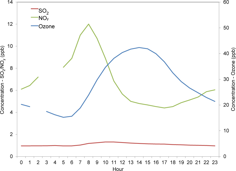
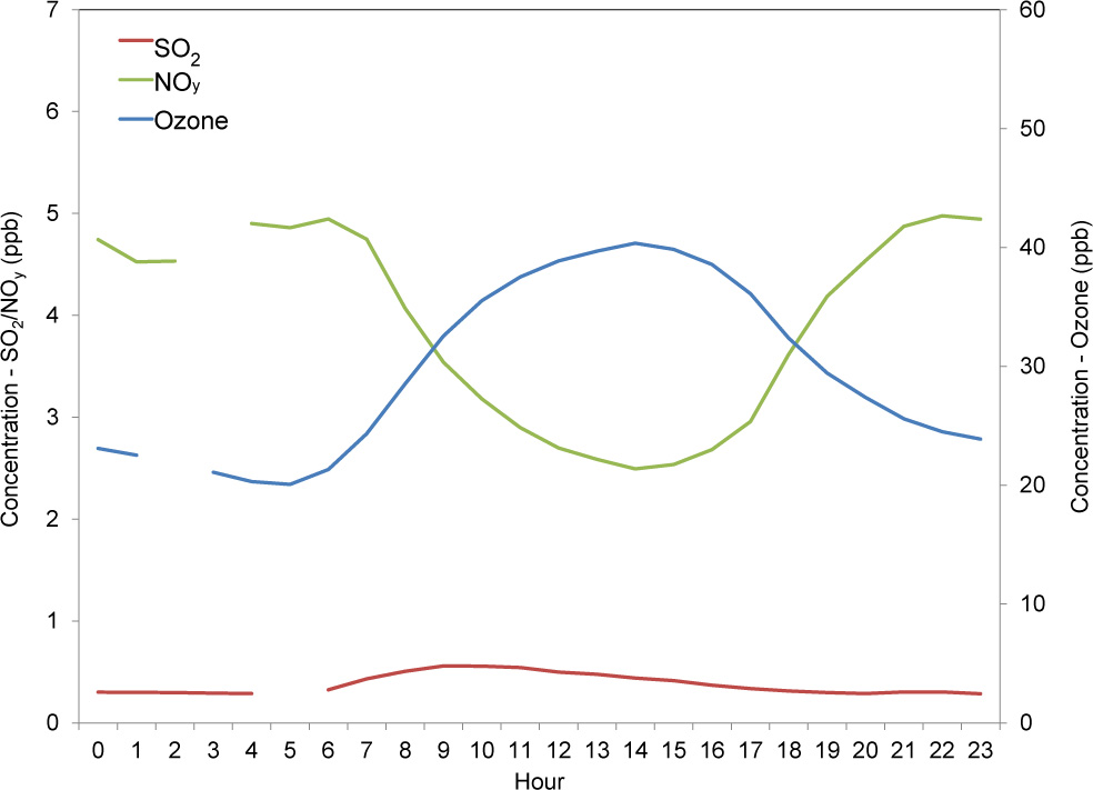
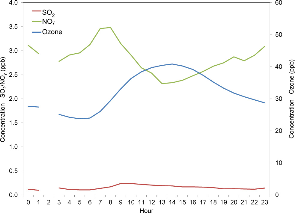
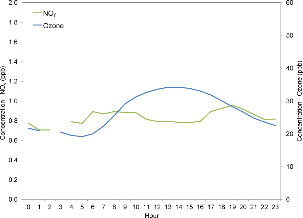
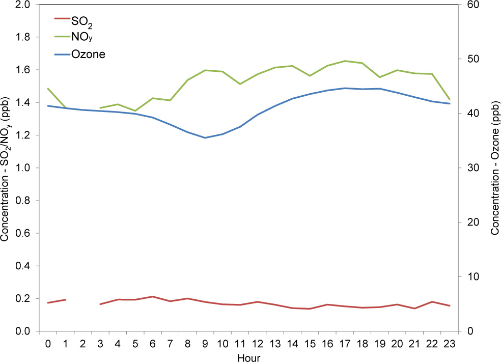
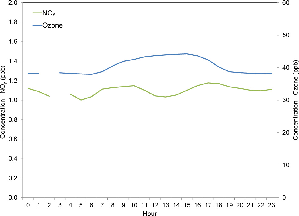
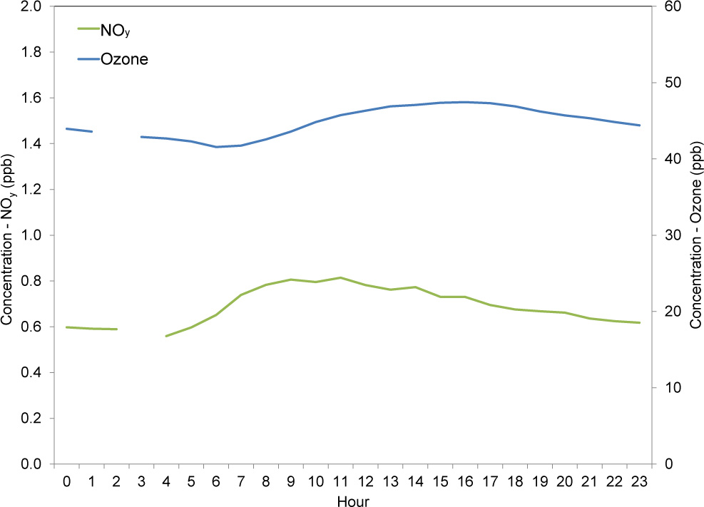
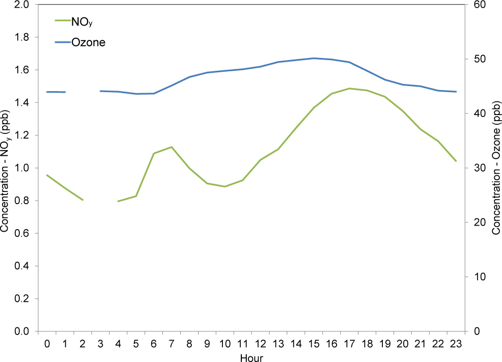
Table 6-2 Summary of 2016 Minimum and Maximum Values from Diurnal Charts
| Site Location | Site Elevation (meters) |
NOy (ppb) | O3 (ppb) | ||
|---|---|---|---|---|---|
| Minimum | Maximum | Minimum | Maximum | ||
| BEL116, MD | 47 | 4.4 | 12.0 | 15 | 42 |
| BVL130, IL | 213 | 2.5 | 5.0 | 20 | 40 |
| MAC426, KY | 243 | 2.3 | 3.5 | 24 | 41 |
| HWF187, NY | 497 | 0.7 | 1.0 | 19 | 34 |
| GRS420, TN | 793 | 1.3 | 1.7 | 36 | 45 |
| PNF126, NC | 1,216 | 1.0 | 1.2 | 38 | 44 |
| PND165, WY | 2,386 | 0.6 | 0.8 | 42 | 47 |
| ROM206, CO | 2,742 | 0.8 | 1.5 | 44 | 50 |
Continuous Trace-level NOy and Ozone
The minimum and maximum mean composite NOy and O3 concentrations shown in Figures 6-2 through 6-9 are summarized in Table 6-2. The sites are listed in order of elevation. The highest NOy concentrations were measured at BEL116, which is situated in an area with numerous mobile-source NOx emissions. Low NOy values (less than 2.0 ppb) were recorded at the five rural sites in New York, Tennessee, North Carolina, Wyoming, and Colorado. The eight profiles in Figures 6-2 through 6-9 illustrate the loss of O3 during the late afternoon and nighttime hours and its production during daylight hours. The diurnal change was less pronounced at the six rural sites. The BEL116 site observed the largest nighttime loss and subsequent highest daytime production, an average difference of about 27 ppb of O3 for 2016. The BVL130 data illustrate a typical diurnal relationship between NOy and O3 concentrations with high NOy concentrations associated with vehicular NOx emissions in the morning and evening and elevated O3 concentrations in the afternoon. The data from the rural MAC426 site also show a diurnal evolution with the highest NOy concentrations in the morning and the evening and highest O3 concentrations in the afternoon. The MAC426 data appear similar to measurements made at an urban site.
Ozone concentrations were also measured at the eight sites listed in Table 6-2 during 2016. The highest O3 concentration (50 ppb) was recorded at ROM206. The concentrations measured at the four sites with the highest elevations show less 24-hour variation than the other four sites because of the dearth of nighttime O3 loss/depletion mechanisms near the high-elevation monitors (Talbot et al., 2005). In particular, nighttime dry deposition is small because fresh nitric oxide is not available to react with O3 and sparse vegetation produces little scavenging. The ROM206 data suggest a production or transport of NOy around sunset. There are no significant NOx sources in the immediate area. The increase in NOy is likely a result of the transformation of polluted air masses from the Front Range Urban Corridor and the frequent late afternoon upslope flow from the east (Baumann et al., 1997).
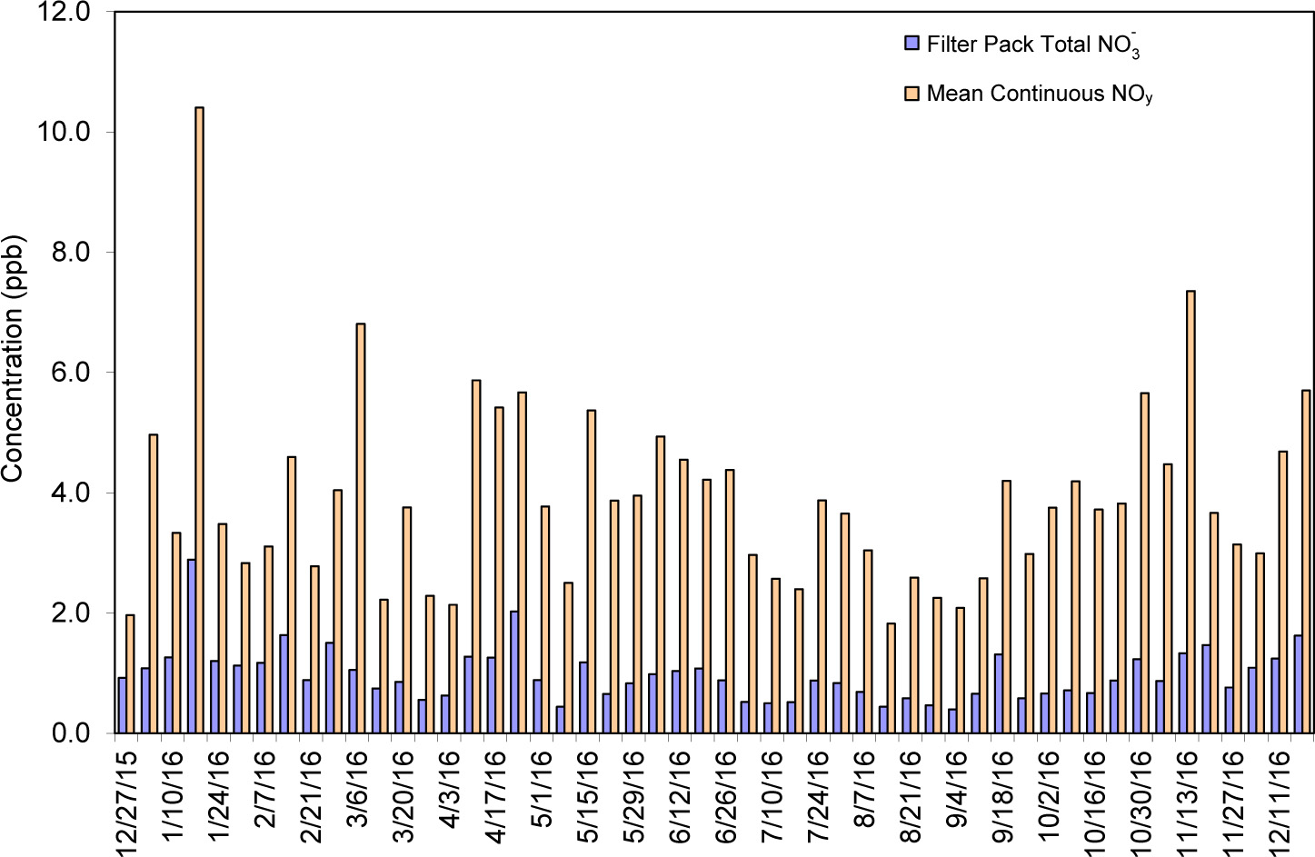
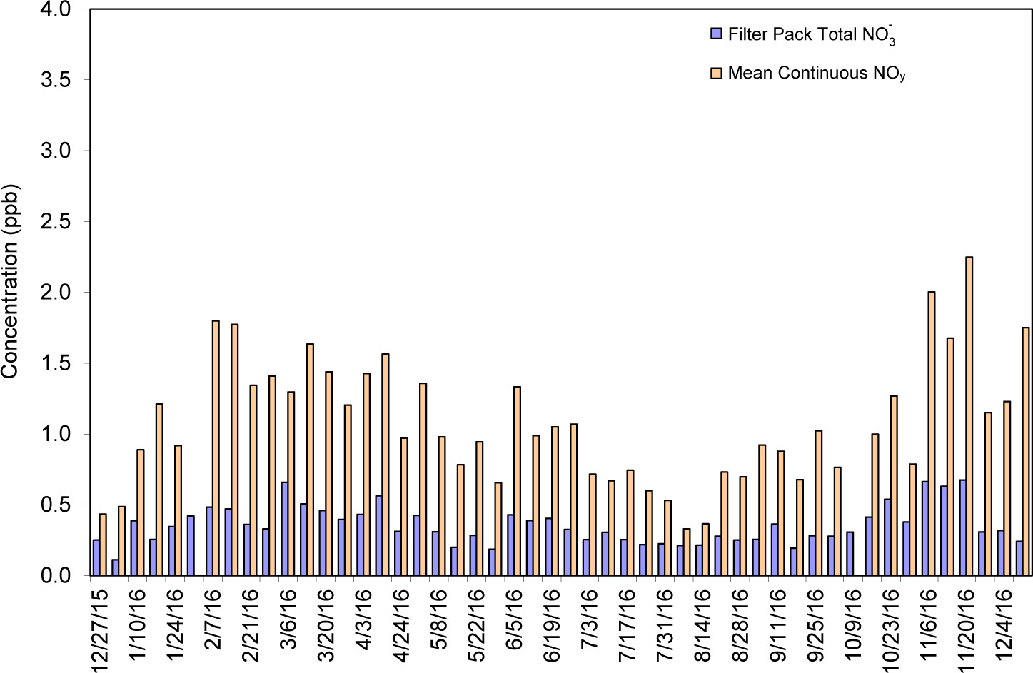
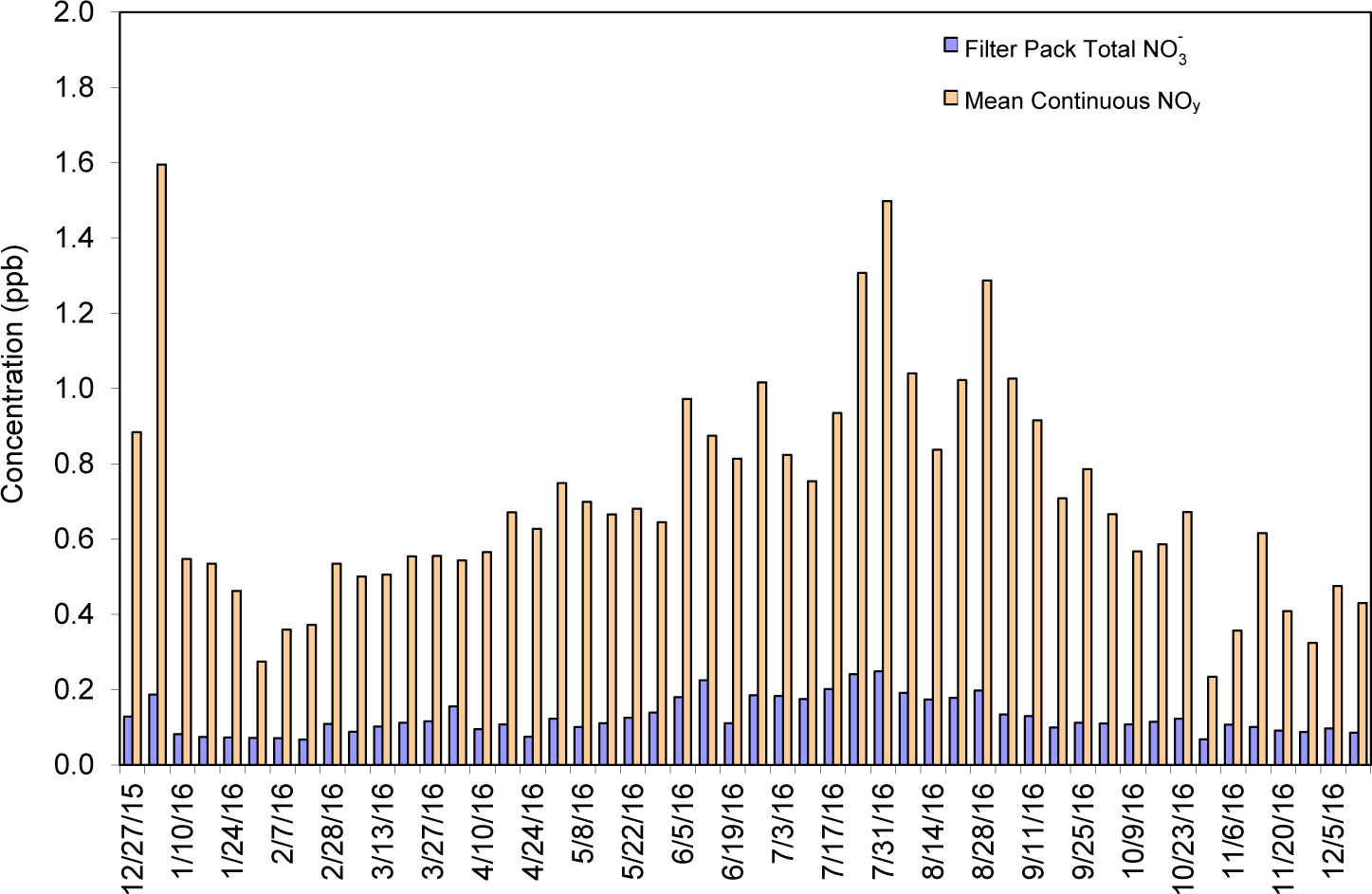
Continuous Trace-level NOy and Filter Pack Total Nitrate Concentrations
Nitric acid and particulate NO3- are measured on CASTNET filter packs, and the sum is reported as total NO3-. Because HNO3 and particulate NO3- are measured as components of NOy, NOy concentrations should always be higher than total NO3- levels (i.e., the ratio of NOy to total NO3- should always be greater than 1.0). A comparison of weekly mean continuous NOy concentrations with filter pack total NO3- levels at BVL130, PNF126, and PND165 for 2016 was used to evaluate the measurements (Figures 6-10 through 6-12). The NOy concentrations were consistently higher than the total NO3- levels, as expected. The results are similar for the other five sites. The weekly total NO3- concentrations, the average weekly NOy levels, and their ratios are listed in Table 6-3. These were calculated as the average of all valid weekly filter pack concentrations, the average of mean NOy values matching the run time of the weekly filter packs, and the average of the ratios calculated for each week. Weekly NOy levels were higher than the weekly total NO3- concentrations with ratios of NOy to total NO3- varying from 2.46 at PNF126 to 10.87 at BEL116. The highest concentration (0.98 ppb) of total NO3- was measured at BVL130.
Figure 6-10 Comparison of BVL130, IL Weekly Mean Continuous Trace-level NOy and Filter Pack Total NO3- Concentrations
 Download Figure
Figure 6-11 Comparison of PNF126, NC Weekly Mean Continuous Trace-level NOy and Filter Pack Total NO3- Concentrations
 Download Figure
Figure 6-12 Comparison of PND165, WY Weekly Mean Continuous Trace-level NOy and Filter Pack Total NO3- Concentrations
 Download Figure
Table 6-3 Summary of Total NO3- and NOy Measurements for 2016
| Site Location | Total NO3- (ppb) | NOy (ppb) | Ratio |
|---|---|---|---|
| BEL116, MD | 0.76 | 8.01 | 10.87 |
| BVL130, IL | 0.98 | 4.39 | 5.03 |
| MAC426, KY | 0.70 | 2.79 | 4.30 |
| HWF187, NY | 0.21 | 0.94 | 3.58 |
| GRS420, TN | 0.45 | 1.97 | 4.93 |
| PNF126, NC | 0.33 | 0.81 | 2.46 |
| PND165, WY | 0.14 | 0.75 | 5.27 |
| ROM206, CO | 0.20 | 1.20 | 5.86 |
Chapter 7: Effects of Wildfires on Air Quality
Wildfires produce large amounts of smoke, fine particulate matter, nitrogen oxides, and other trace-level gases. In particular, in the western United States, wildfires and prescribed agricultural and forest management burns are large sources of aerosols and trace gases. The 2016 western wildfire season was extensive, especially following the winter of 2015–2016 drought. The Maple Fire at the western edge of Yellowstone National Park burned over 45,000 acres in August 2016. Fine particulate matter concentrations measured at IMPROVE sites in and near the park showed elevated concentrations. The Jack Fire in Arizona started on May 29, 2016 and continued to burn until July 1. During that period, it burned 33,850 acres in the Coconino National Forest, which is located about 24 kilometers south of Flagstaff.
Wildfires occur naturally in the United States. In the West, wildfires and prescribed agricultural and forest management burns are a large global source of aerosols and trace-level gases from burning vegetation, buildings, and other materials. Smoke from wildfires is a significant source of air pollution and can pose potential risks to health, visibility, and safety. According to Liu et al. (2016), open fires contributed significantly (about 37 percent) to PM2.5 emitted in the contiguous United States and produced substantial amounts of O3 precursors. Wildfires usually consume more biomass fuel per unit area burned than prescribed fires. Land use changes, wildfire management strategies, and climate change have increased wildfire size and frequency and the length of the fire season in the western United States. The 2016 western wildfire season was extensive in both area burned and length of the season, especially following the drought during the winter of 2015–2016.
Liu et al. (2016) analyzed aircraft air pollutant measurements in three plumes from wildfires in the western United States in 2013. The study reported an extensive set of emission factors for about 80 gases and five components of submicron particulate matter (PM1) from these wildfires. The measured emission factors were used to estimate the annual wildfire emissions of CO, NOx, total non-methane organic compounds, and PM1 from 11 western states. The wildfires emitted high amounts of PM1 with organic aerosol dominating the mass. The results from Liu et al. (2016) indicate that PM1 emissions from wildfires are substantially higher than those from prescribed burns and that prescribed burning may be an effective method to reduce overall fine particle emissions.
Measurements from CASTNET, IMPROVE, the EPA Chemical Speciation Network (CSN), and other federal and state networks provide information to characterize the impacts of wildfires on air quality and visibility near critical resources such as national parks. In 2016, fires extended from the northern tier states to Arizona, New Mexico, and Texas. Figure 7-1 gives box plots of third quarter mean O3 measurements aggregated over the CASTNET western reference sites (Appendix A). The O3 box plots were constructed by averaging all valid hourly O3 concentrations within third quarter by site and then averaging those averages for all western reference sites. The figure shows increased aggregated mean concentrations for 2016.
Figure 7-1 Trends in Third Quarter Mean O3 Concentrations at CASTNET Western Reference Sites
 Download Figure
During the 2016 fire season, 22 fires burned in Yellowstone National Park, WY (YEL408). The park is required to protect human life as well as the approximately 2 percent of Yellowstone’s 2.2 million acres that are considered developed (e.g., roads, buildings, and other infrastructure) from the threat of fire, while at the same time letting fire play its ecological role in the landscape as much as possible. 2016 was the most active fire year since 1988 with 62,000 acres burned. Seven wildfires were the result of human activity such as a campfire, vehicle operation, or cigarettes. The remainder of the 2016 wildfires resulted from natural causes (i.e., lightning). Eleven fires were suppressed because infrastructure was threatened. Many fires were managed to allow them to perform their natural role in the ecosystem. The largest of these fires, the Maple Fire, burned over 45,000 acres.
Figure 7-2 is a photograph of the Maple Fire in Wyoming, August 21, 2016, taken by the Visible Infrared Imaging Radiometer Suite (VIIRS) instrument aboard the National Oceanic and Atmospheric Administration (NOAA)/National Aeronautics and Space Administration (NASA) Suomi National Polar- orbiting Partnership satellite. The Maple Fire was detected the evening of August 8, 2016 by an aircraft passing over Yellowstone. The fire was located 6 kilometers (km) east of the park’s west boundary, 8 km northeast of the community of West Yellowstone, MT, and 4.5 km from Madison Junction. Rain accompanied by cool weather at the end of August slowed the spread of the Maple Fire that had come within 5 km of West Yellowstone.
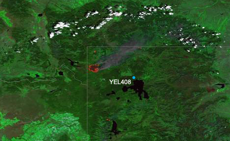
Hourly and DM8A O3 concentrations measured at three Wyoming CASTNET sites [Basin (BAS601), Pinedale (PND165), and YEL408] over the period of August 11, 2016 through September 6, 2016 are plotted in Figure 7-3. Time series of PM2.5 concentrations measured over the period July 8, 2016 through October 6, 2016 at IMPROVE sites in Wyoming [Boulder Lake (BOLA1), Bridger Wilderness (BRID1), North Absaroka (NOAB1), and Yellowstone (YELL2)] are shown in Figure 7-4. Comparatively high PM2.5 concentrations were measured at YELL2 and NOAB1 after the fire started. For example, PM2.5 concentrations were 2.92 times higher at NOAB1 and 2.59 times higher at YELL2 during the period of the Maple Fire than they were during the remainder of July through August. Concentrations were reduced by the end of the month.
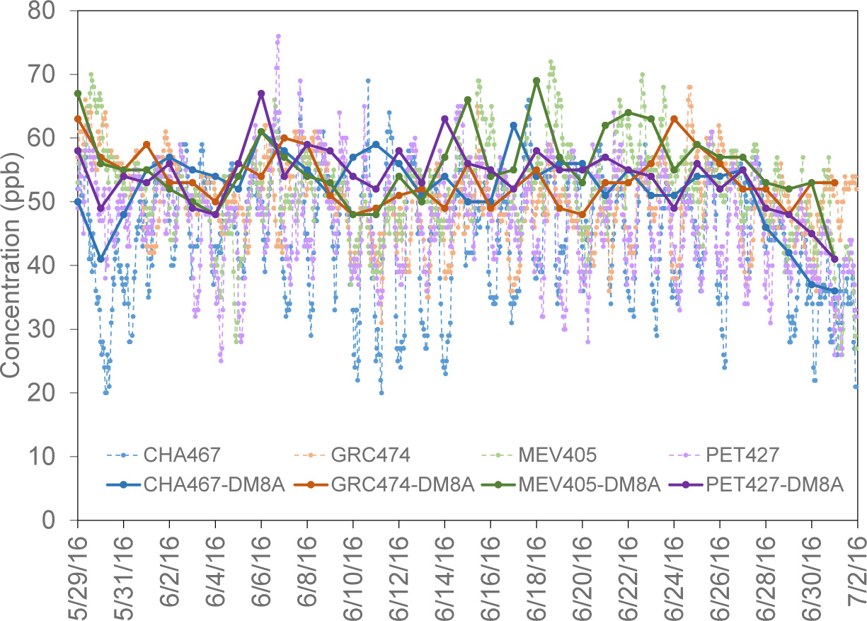
Lightning started the Jack Fire in Arizona on May 29, 2016, and it continued to burn until July 1. During that period, it burned 33,850 acres in the Coconino National Forest, which is located about 24 km south of Flagstaff, 113 km south-southeast of the CASTNET site at Grand Canyon National Park (GRC474), and 145 km west of the CASTNET site at Petrified National Forest (PET427). Figure 7-5 shows smoke from the Jack Fire streaming eastward. Weekly average O3 concentrations shown in Figure 7-6 for three CASTNET sites in Arizona [GRC474, PET427, and Chiricahua National Monument (CHA467)] and one in Colorado [Mesa Verde National Park (MEV405)] showed no significant change after the beginning of the Jack Fire. Time series of PM2.5 concentrations measured over the period April 30, 2016 through July 29, 2016 at nearby IMPROVE sites Grand Canyon (GRCA2), Petrified National Forest (PEFO1), Chiricahua (CHIR1), and Mesa Verde National Park (MEVE1) are shown in Figure 7-7. Fine particulate matter concentrations measured at PEFO1 and CHIR1 were elevated during the fire except for relative minima for two samples on June 14 and June 17, 2016. Synoptic weather data (NOAA National Centers for Environmental Prediction, 2018) suggest the wind direction shifted southeast during those two sampling periods, transporting the fire plume away from the samplers at PEFO1 and CHIR1. PM2.5 concentrations were 1.5 times higher at CHIR1 and 2.25 times higher at PEFO1 during the period of the Jack Fire than during the remainder of April through July.
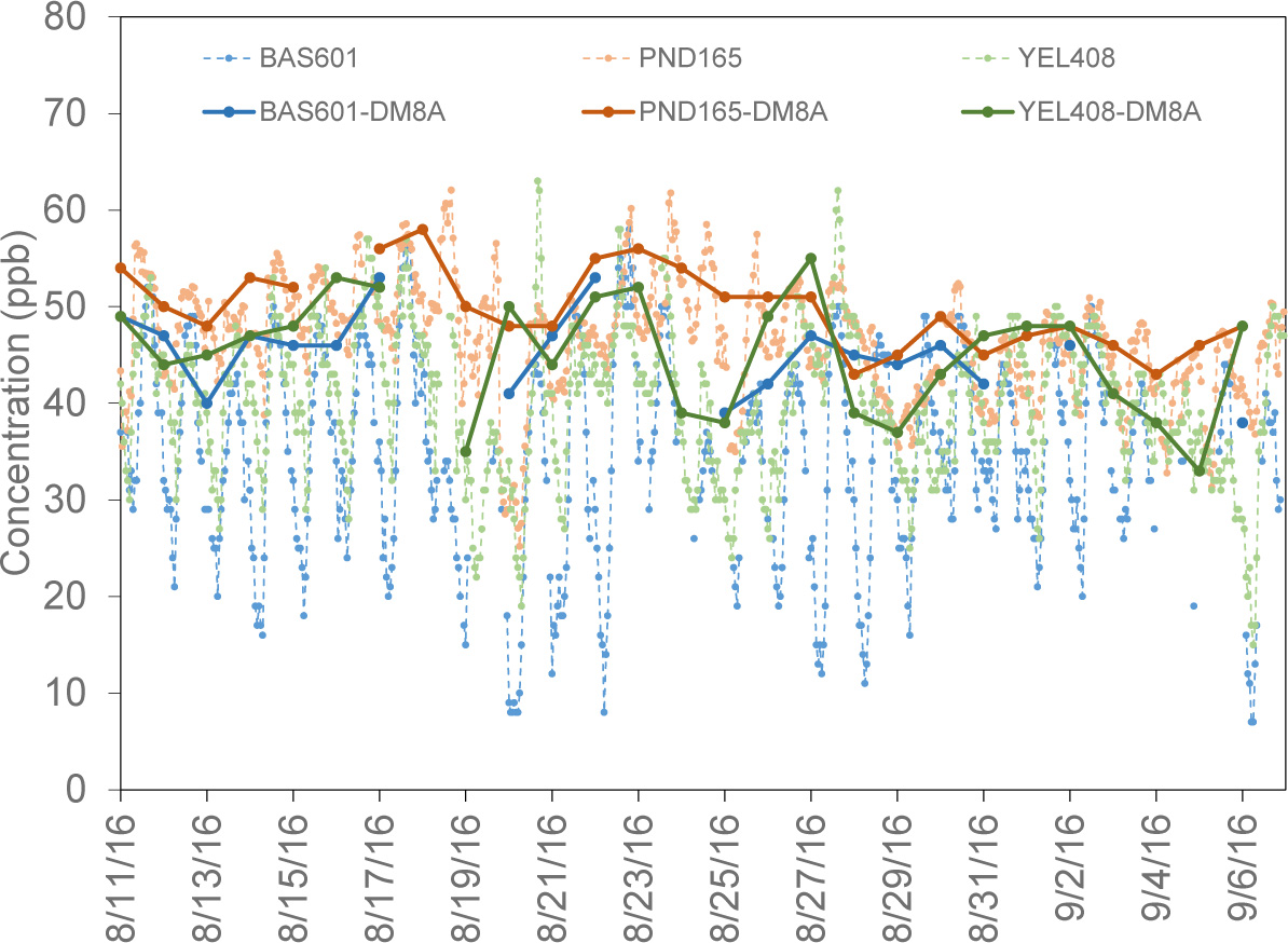
Figure 7-4 Time Series of Wyoming IMPROVE PM2.5 Data
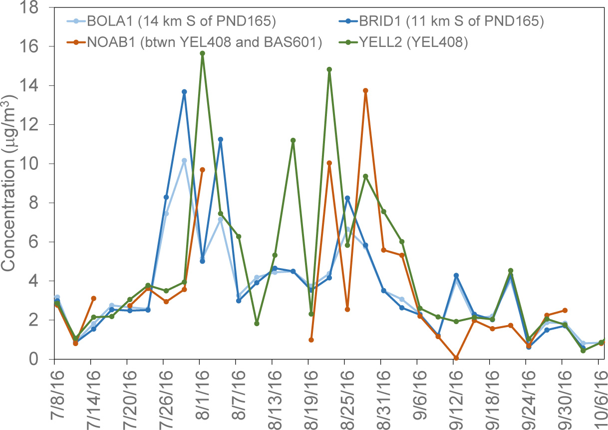
Note: Corresponding CASTNET site with the location of the IMPROVE site in relation to the CASTNET site listed in parentheses.
Download FigureFigure 7-5 Satellite photo of Arizona Jack Fire June 9, 2016
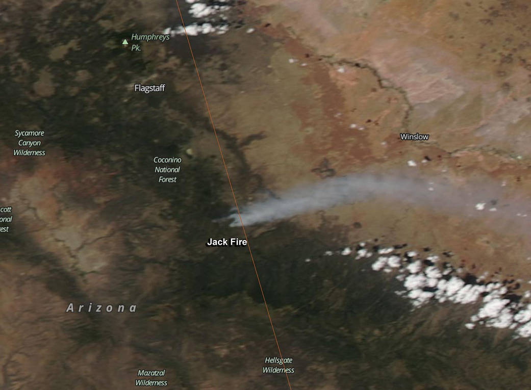
Source: NASA (2016), LANCE/EOSDIS MODIS Rapid Response Team, GSFC
Download FigureFigure 7-6 Time Series of CASTNET O3 Data for Sites in Arizona (PET427 GRC474, CHA467) and Colorado (MEV405)
 Download Figure
Figure 7-7 Time Series of IMPROVE PM2.5 Data for Sites in Arizona (PEF01, GRCA2, CHIR1) and Colorado (MEVE1)
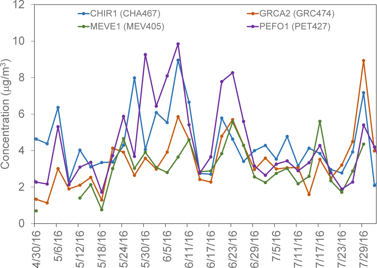
Note: IMPROVE sites are approximately co-located with the corresponding CASTNET site listed in parentheses. Download Figure
Chapter 8: Atmospheric Deposition of Nitrogen
CASTNET was designed to provide estimates of the dry deposition of nitrogen and sulfur pollutants across the United States. To assess the status of dry and total deposition for 2016, EPA used NADP’s Total Deposition Science Committee Hybrid Method. The hybrid method combines measured pollutant concentrations with output from the CMAQ modeling system. Total deposition was calculated as the sum of estimated dry and wet deposition.
Gaseous and particulate nitrogen pollutants are deposited to the environment through dry and wet atmospheric processes. A primary goal of CASTNET is to estimate the dry deposition of pollutants from the atmosphere to sensitive ecosystems. The NADP Total Deposition Science Committee (TDep) Hybrid Method (EPA, 2015d; Schwede and Lear, 2014) combines CASTNET monitoring data with output from the CMAQ modeling system (Byun and Schere, 2006) to estimate dry deposition. The TDep method gives priority to using measurement data from air quality monitoring sites when available and to CMAQ output in areas where monitoring data are not available. In addition, CMAQ provides modeled data for species that are not routinely measured. The TDep method and its recent updates are discussed on the TDep web page. See also the NADP Fact Sheet, “Hybrid Approach to Mapping Total Deposition.”
The TDep method estimates wet deposition using PRISM to develop a continuous grid of precipitation data. PRISM uses terrain elevation, slope, and aspect and climatic measurements to estimate precipitation. Pollutant concentrations in precipitation, which were estimated for the PRISM grid, were provided by NADP/NTN. The concentration and precipitation grids were merged in order to estimate pollutant wet deposition rates. Dry and wet deposition fluxes were added to obtain estimates of total deposition, which are presented on the maps in this chapter as kilograms per hectare per year (kg ha -1 yr -1 ).
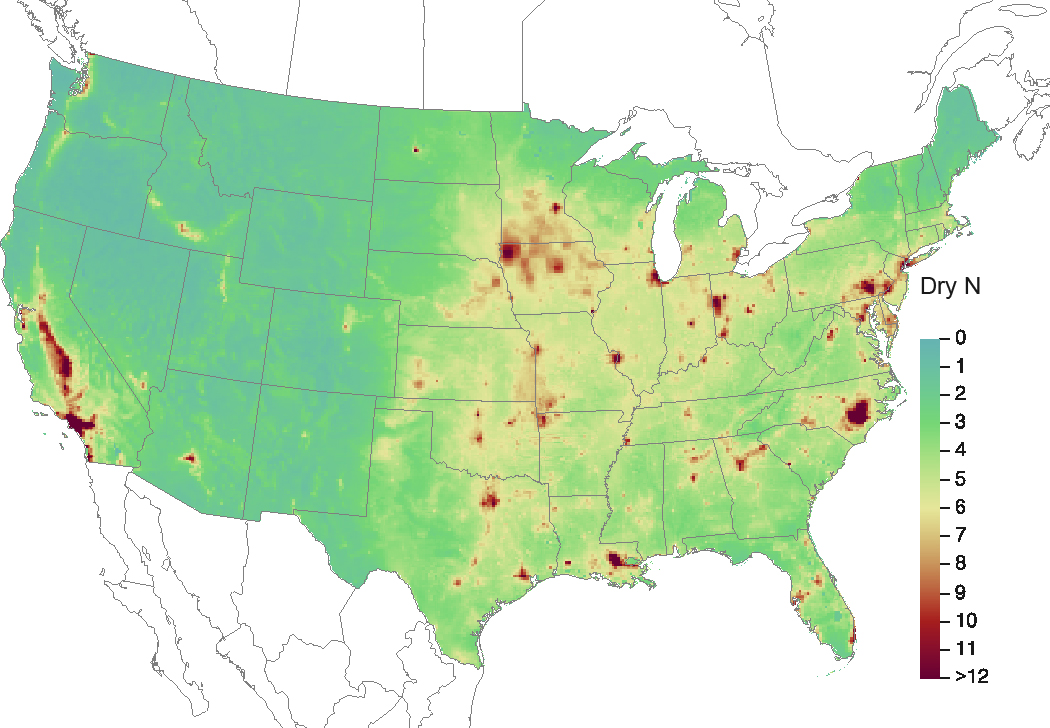
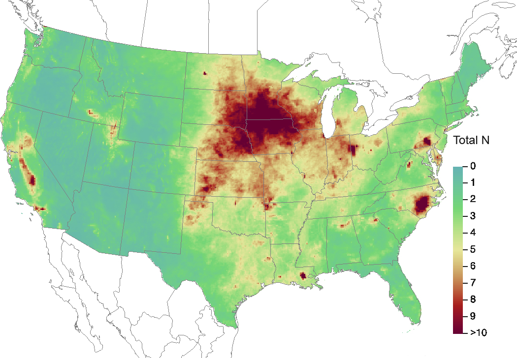
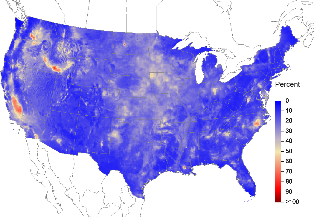
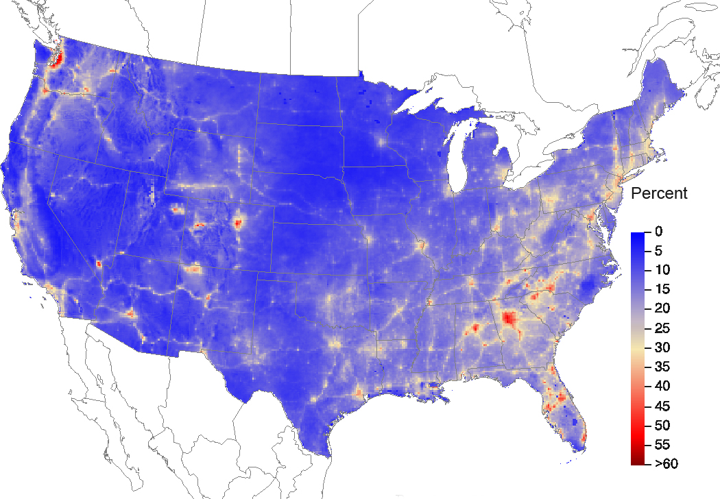
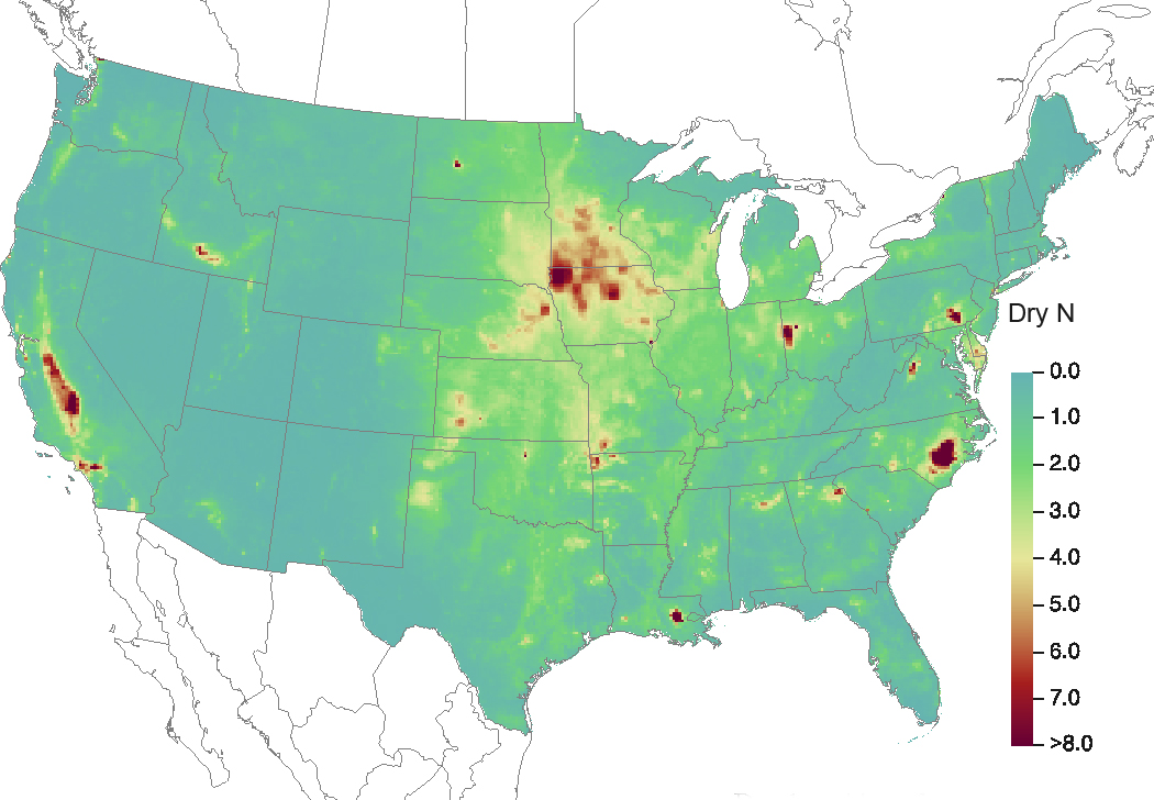
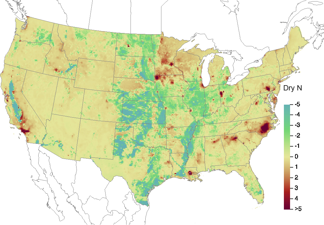
Figure 8-1 illustrates TDep method estimates of dry fluxes of nitrogen (N) for 2016. The magnitude of the deposition fluxes is illustrated by the shading in the figure legend. A map of total deposition of N for 2016 is given in Figure 8-2. The percentage of total deposition of N due to dry deposition is shown in Figure 8-3. A map of TDep method estimates of total deposition of reduced N species for 2016 is given in Figure 8-4. Figure 8-5 gives the percentage of reduced N species from dry deposition. Dry deposition of N species that are not routinely measured but are estimated by the TDep method is shown in the map in Figure 8-6. The percentage of total deposition of N that is not measured directly but is calculated by the TDep method is shown in Figure 8-7. Annual gross dry deposition of NH3 for 2016 is shown in Figure 8-8, and the net dry deposition of NH3 is given in Figure 8-9.
Figure 8-1 TDep Dry Deposition Estimates of N (kg ha -1 yr -1) for 2016
Source: CASTNET|CMAQ|NADP/NTN
Download FigureFigure 8-2 TDep Total Deposition Estimates of N (kg ha -1 yr -1) for 2016
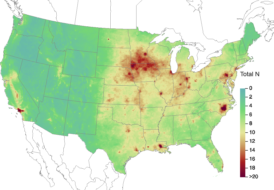
Source: CASTNET|CMAQ|NADP/NTN
Download FigureFigure 8-3 TDep Percent of Total Deposition of N from Dry Deposition for 2016
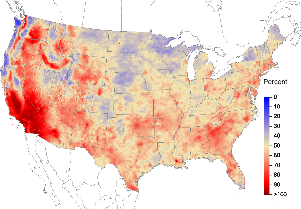
Source: CASTNET|CMAQ|NADP/NTN
Download FigureFigure 8-4 TDep Total Deposition Estimates of Reduced N Species (kg ha -1 yr -1) for 2016
Source: CASTNET|CMAQ|NADP/NTN
Download FigureFigure 8-5 TDep Percent of Total Deposition of Reduced N Species from Dry Deposition for 2016
Source: CASTNET|CMAQ|NADP/NTN
Download FigureFigure 8-6 TDep Dry Deposition Estimates of Unmonitored N Species (kg ha -1 yr -1) for 2016
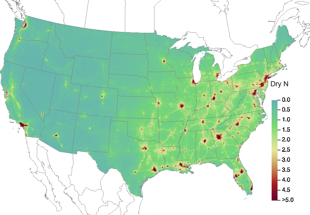
Source: CASTNET|CMAQ|NADP/NTN
Download FigureFigure 8-7 TDep Percent of Total Deposition of N from Dry Deposition of Unmonitored Species for 2016
Source: CASTNET|CMAQ|NADP/NTN
Download FigureFigure 8-8 TDep Gross Dry Deposition of NH3 as N (kg ha -1 yr -1) for 2016
Source: CASTNET|CMAQ|NADP/NTN
Download FigureFigure 8-9 TDep Net Dry Deposition of NH3 as N (kg ha -1 yr -1) for 2016
Source: CASTNET|CMAQ|NADP/NTN
Download FigureChapter 9: Monitoring on Whiteface Mountain during 2015 and 2016
Continuous, trace-level, gaseous air quality monitors and filter pack samplers were run at two CASTNET sites on Whiteface Mountain during 2015 and 2016. The measurements at these sites were performed to (1) analyze differences in air quality resulting from variance in elevation and exposure and to (2) provide data to understand atmospheric processes such as ozone formation.
Whiteface Mountain in the Adirondack Mountains in upstate New York has been the site of many research studies over the decades and has a long history of atmospheric chemistry measurements. A CASTNET small footprint filter pack site (WFM105) was installed near an NTN precipitation collector in 2012. This location is also known as the Marble Mountain Lodge site and sits on the eastern shoulder of the Whiteface massif at an elevation of 604 meters. A seasonal CASTNET small footprint site, WFM007, was installed at the Summit Observatory location in 2015 and usually operates from May or June through September or October, as conditions allow. The Summit Observatory is at the peak of the mountain at 1,483 meters. Continuous O3, NO2, NO, and SO2 have been measured at both locations since the late 1980s. The continuous data used in this chapter were provided by the Atmospheric Sciences Research Center (ASRC) of the State University of New York and the New York State Energy Research and Development Authority (NYSERDA).
Weekly filter pack concentrations of SO42-, SO2, NO3-, NH4+, HNO3-, and Ca 2+ from WFM105 and WFM007, the lodge and summit sites, respectively, were compared for 2015 and 2016 during the warm season from the onset of sampling at the summit location in the spring until the site was closed for the season in the fall. Additionally, continuous SO2 and filter pack SO2 data from both locations were analyzed during the period of operation for the summit location. Continuous O3, NO, and NO2 data, which are available year-round from both sites, were compared for 2015 and 2016 (ASRC, 2017).
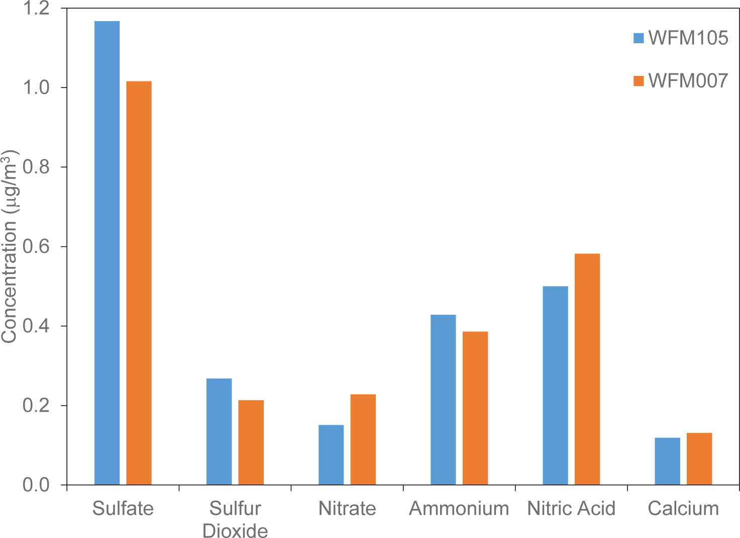
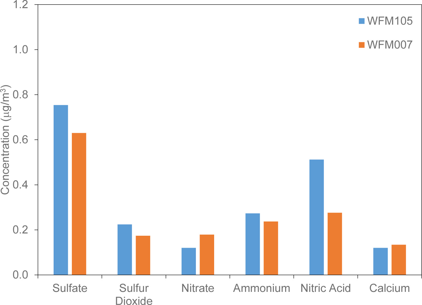
Figures 9-1 and 9-2 depict seasonal average filter pack concentrations of SO42-, SO2, NO3-, NH4+, HNO3-, and Ca 2+ for 2015 and 2016 at both WFM105 and WFM007. Sulfate, SO2, and NH4+ seasonal concentrations were higher at WFM105 than WFM007 for both years, with the 2015 concentrations being higher than the 2016 concentrations. The WFM007 summit site had higher concentrations of NO3-, HNO3-, and Ca 2+ than WFM105 in 2015. Comparisons were similar in 2016 with the exception that HNO3- concentrations were higher at WFM105.
Concentrations were higher in 2015 than 2016 at WFM105 with the exceptions of HNO3- and Ca 2+ , which had similar concentrations (0.5 μg/m 3 versus 0.512 μg/m 3 for HNO3- and 0.119 μg/m 3 versus 0.12 μg/m 3 for Ca 2+ ) for both years. The 2015 concentrations were greater than 2016 concentrations at WFM007 for all analytes.
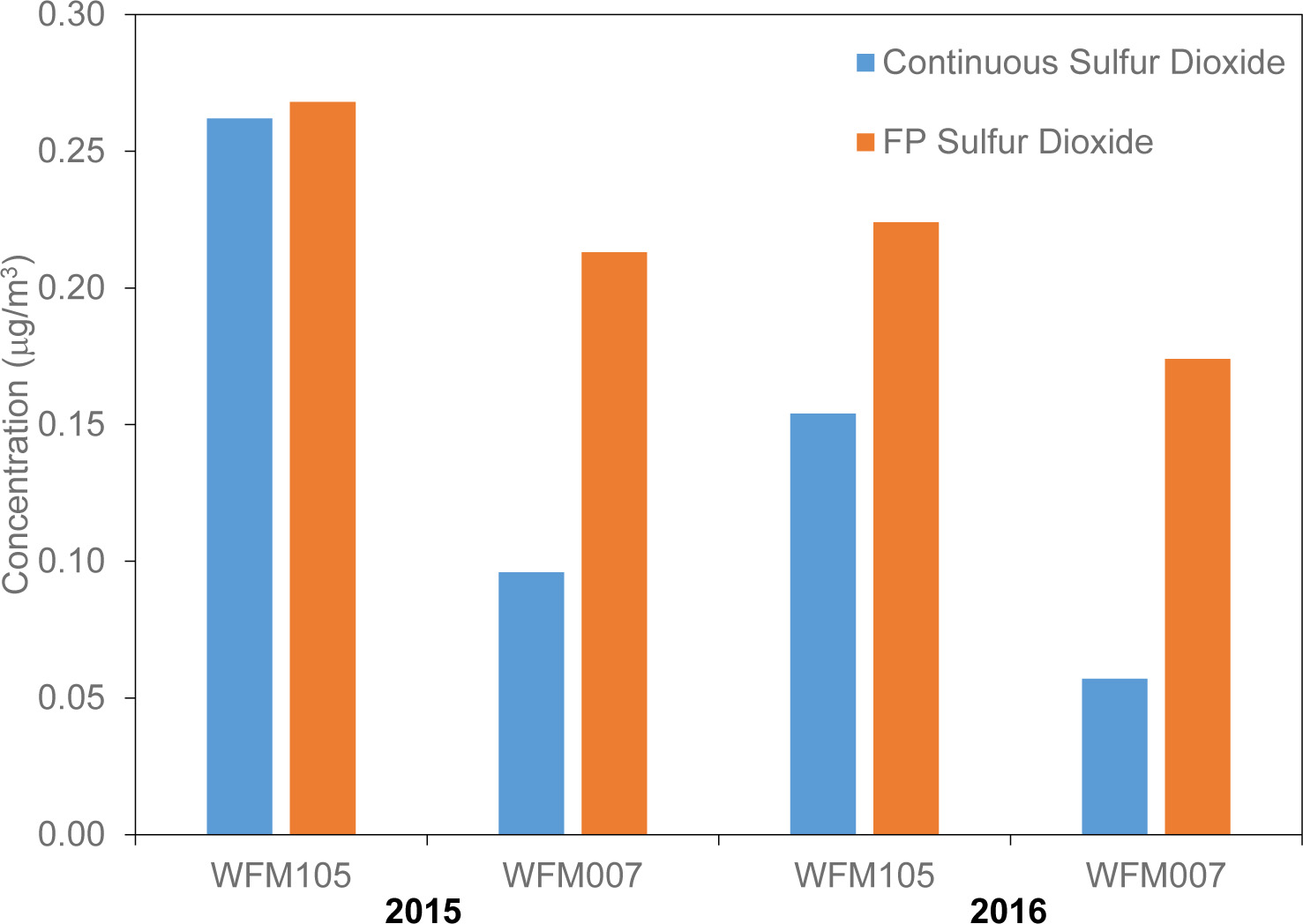
Sulfur dioxide and SO42- are both produced by SO2 emissions. The ratio of SO42- to SO2 is a measure of the age of the polluted air mass. Higher SO42- concentrations relative to SO2 levels measured at both sites suggest that air pollution measured at Whiteface Mountain was produced during transport from distant pollutant sources.
Figure 9-3 shows seasonal filter pack and continuous SO2 concentrations from both locations for 2015 and 2016. The filter pack SO2 concentrations were higher than the continuous concentrations at both sites during both years. The 2015 seasonal concentrations for filter pack and continuous SO2 were higher than the 2016 seasonal concentrations.
Figure 9-3 Warm Season Filter Pack and Continuous SO2 Concentrations at WFM105 and WFM007 for 2015 and 2016
 Download Figure
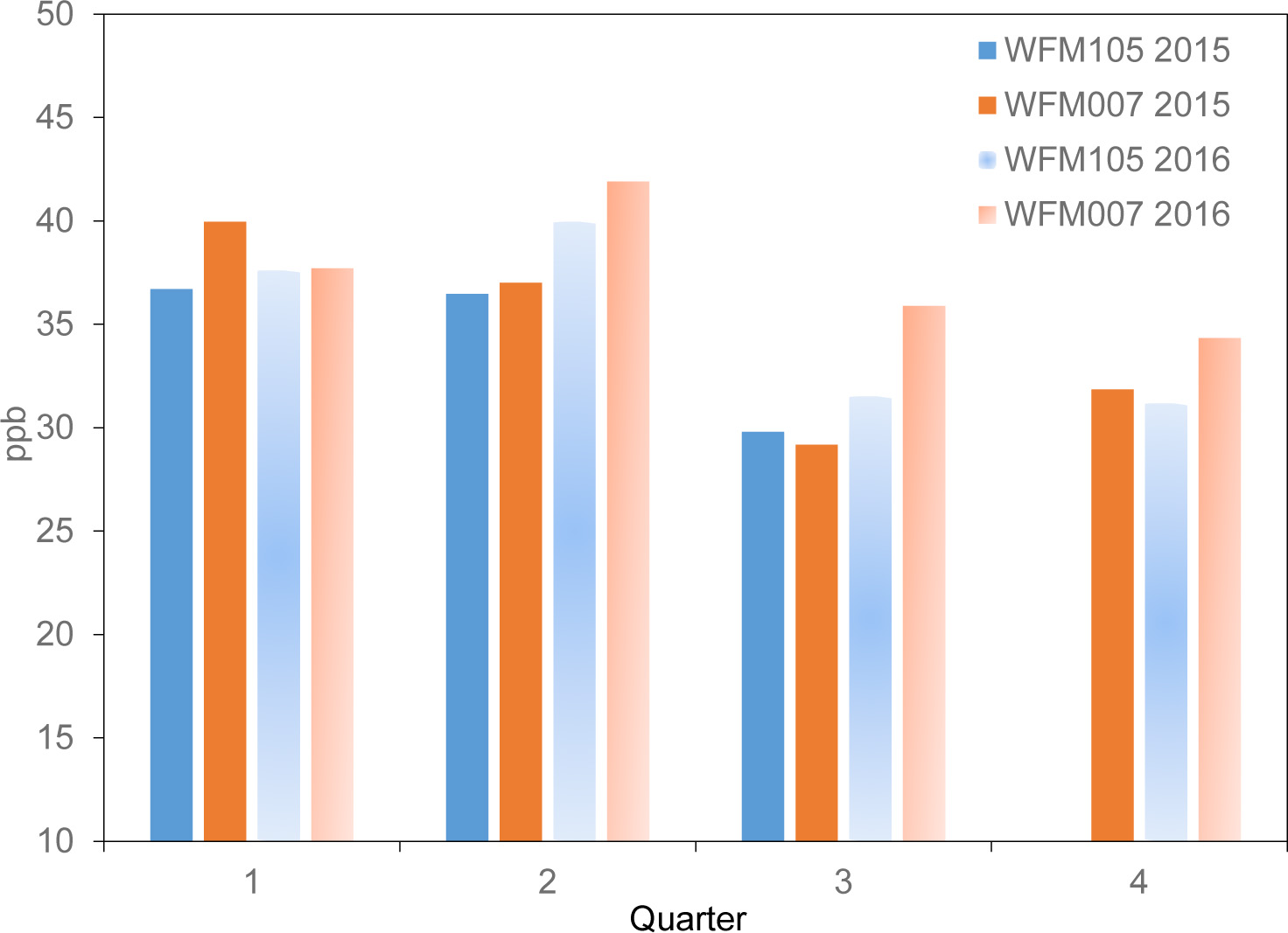
Quarterly averages of O3 for both years and both sites are presented in Figure 9-4. WFM007 generally had higher quarterly averages than WFM105 with exception of third quarter 2015. Quarterly O3 averages were greater in 2016 than 2015 at both sites with the exception of the first quarter for WFM007. Ozone values were not available for fourth quarter 2015 for WFM105.
Figure 9-4 Quarterly Average O3 Concentrations for WFM105 and WFM007 for 2015 and 2016
 Download Figure
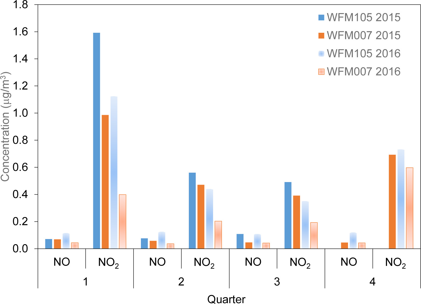
Continuous NO and NO2 quarterly average concentrations for both sites for 2015 and 2016 are plotted in Figure 9-5. WFM105 measured higher quarterly averages of NO and NO2 than WFM007 for both years. Data were not available for fourth quarter 2015 from WFM105.
Nitrogen dioxide concentration values for 2015 at WFM105 were greater with respect to the 2016 values. However, the 2015 NO concentration values at WFM105 were lower than 2016 for the first and second quarters and equal for the third quarter. Concentrations of both analytes were greater at WFM007 in 2015 than 2016.
Diurnal plots of O3, NO, and NO2 for both locations for the 2007 and 2016 warm seasons are shown in Figures 9-6 through 9-9. Data from 2007 were selected to illustrate the changes in air quality over a 10-year period. The O3 and NO2 concentrations were higher at WFM007 in 2007 than at WFM105. While NO values were about equivalent at the two sites, WFM105 had a higher diurnal peak. There was no discernible diurnal pattern for O3 in 2007 at WFM007, but both locations showed a midday minimum for NO2 due to conversion to O3 by daytime photochemical processes.
Ozone values were again greater at WFM007 than WFM105 in 2016. However, the NO2 values were lower at WFM007 with respect to the WFM105 site. The NO concentrations were also lower at the WFM007 site. The 2016 NO2 concentrations at WFM105 again showed a midday peak for ozone and a dip for NO2; WFM007 showed a slight midday decline for both parameters.
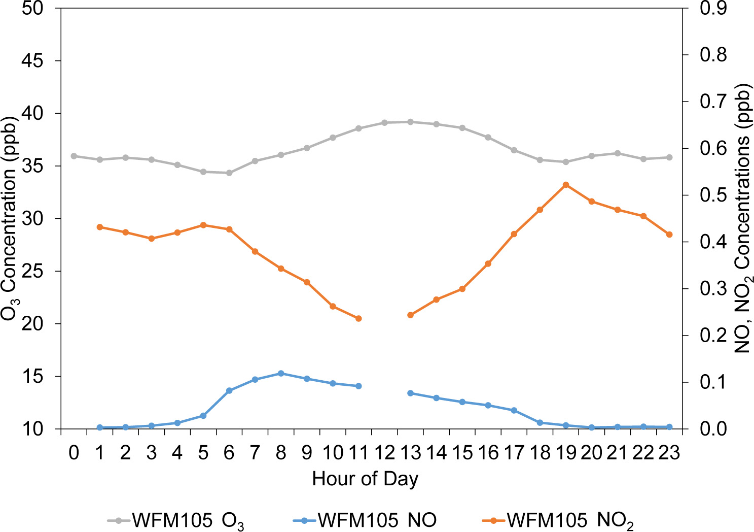
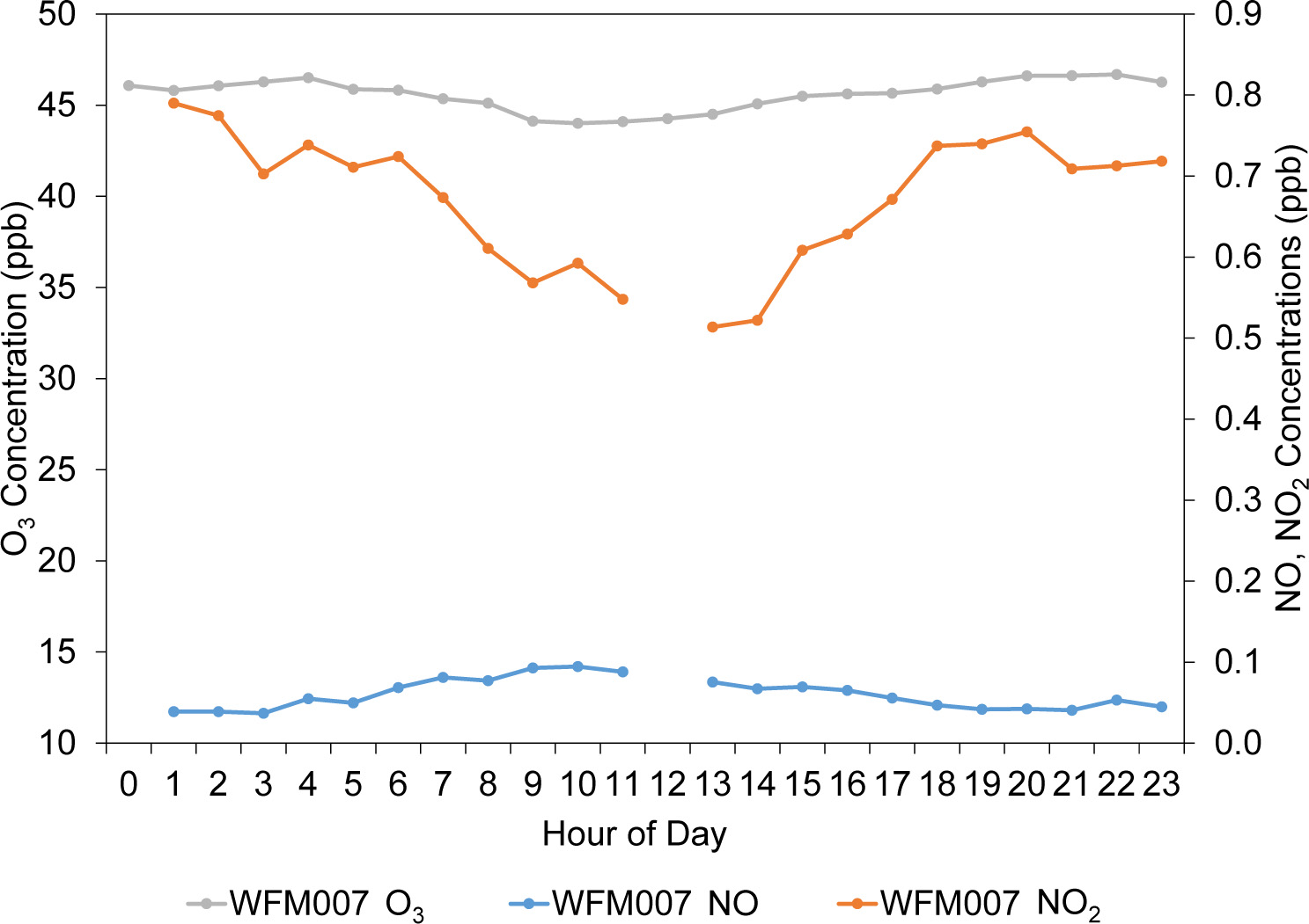
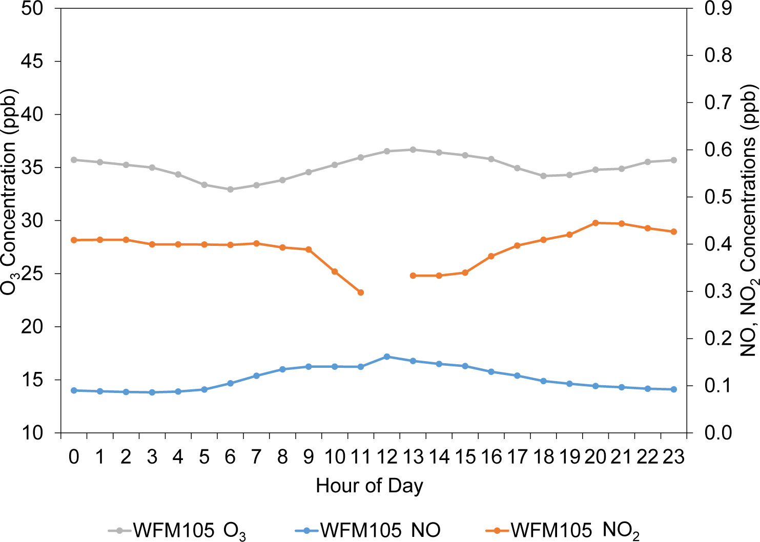
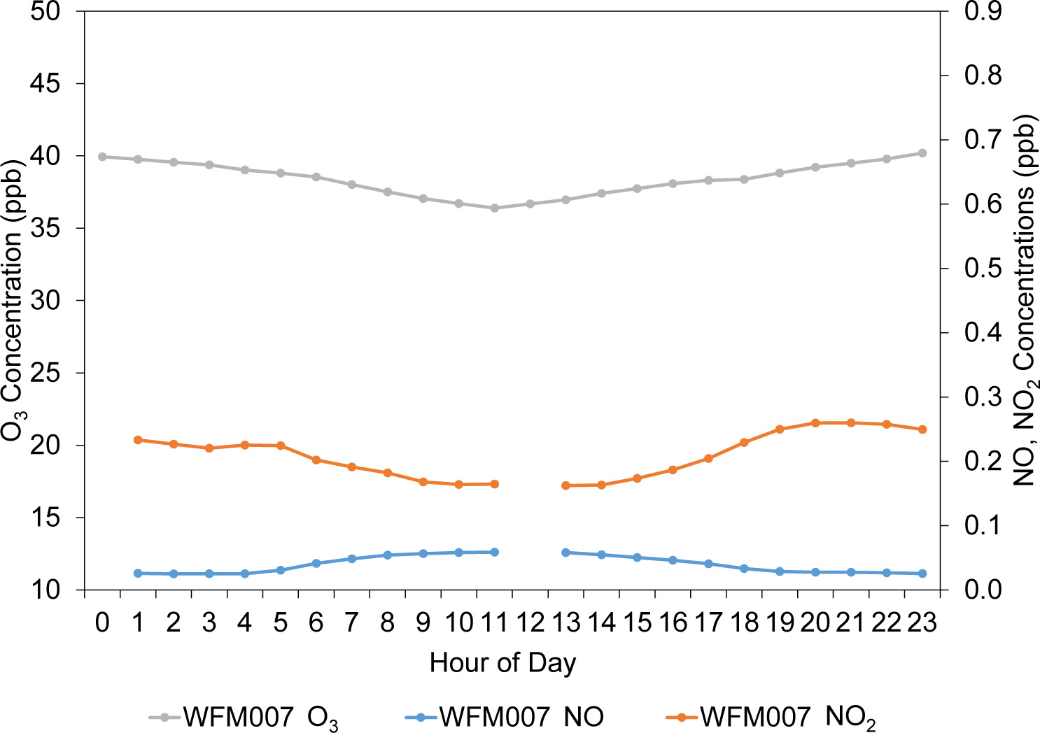
The 2016 average warm season NO and NO2 concentrations were higher than the 2007 warm season averages at WFM105, while the 2016 O3 average was slightly lower (37 ppb in 2007 versus 35 ppb in 2016). This pattern was reversed at the summit, WFM007, where the 2016 warm season averages of all three analytes were lower than the 2007 averages.
Figures 9-10 and 9-11 show O3 concentrations for both Whiteface Mountain locations for 2015 and 2016 and for the nearby, lower elevation CASTNET site at Huntington Wildlife Forest, NY (HWF187) to provide a more detailed analysis of the diurnal pattern for O3 and to illustrate the significant diurnal change of O3 at lower elevations.
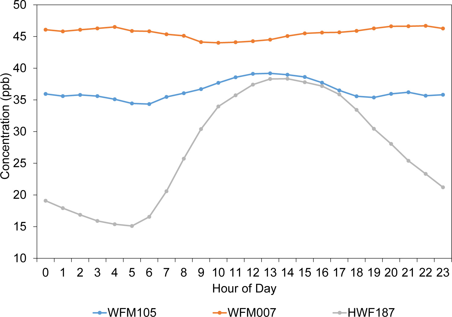
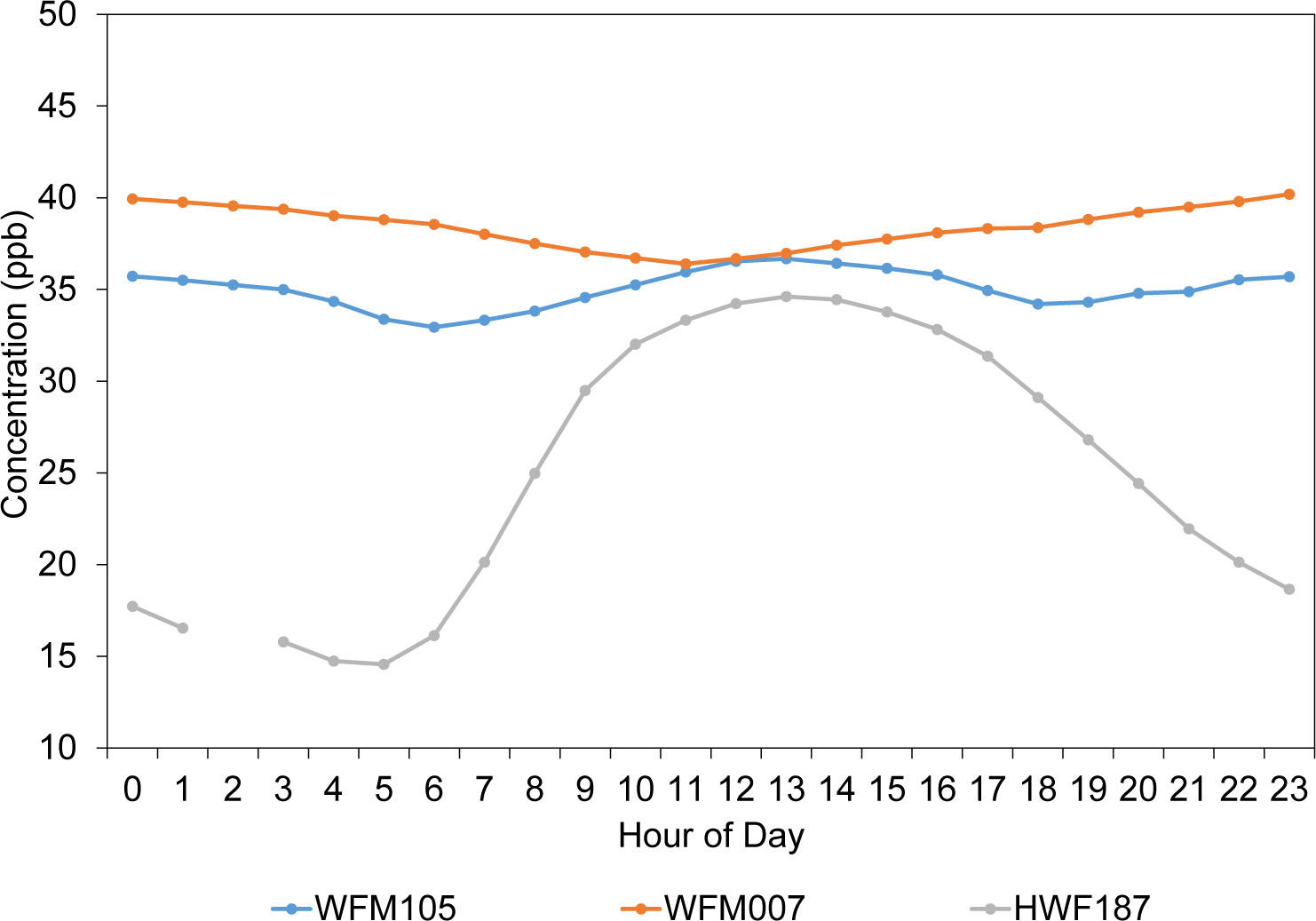
Ozone levels were are highest at WFM007, the summit, and showed little diurnal variation, most likely due to a lack of depletion mechanisms, e.g., little vegetation to produce dry deposition and no fresh NO to scavenge O3. WFM105 ozone values were greater than those at HWF187. A slight diurnal pattern was discernible at WFM105, but it was not as pronounced as the diurnal patterns seen at HWF187, which exhibited a diurnal change of around 20 ppb daily.
Chapter 10: Atmospheric Deposition of Sulfur, Base Cations, and Chloride
CASTNET was designed to provide estimates of the dry deposition of nitrogen and sulfur pollutants, base cations, and chloride across the United States. EPA used the NADP TDep method to assess the status of dry and wet deposition for 2016. Total deposition was calculated as the sum of estimated dry and wet deposition.
Gaseous and particulate sulfur pollutants, base cations, and chloride are deposited to the environment through dry and wet atmospheric processes. A principal goal of CASTNET is to estimate the rate of dry deposition of these compounds from the atmosphere to sensitive ecosystems. The NADP TDep method (EPA, 2015d; Schwede and Lear, 2014) was used to estimate dry and wet deposition. Dry and wet deposition rates were summed to obtain total deposition across the United States.
Sulfur Deposition
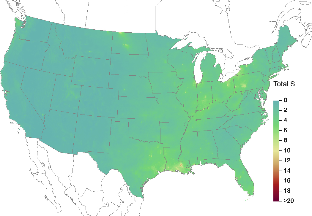
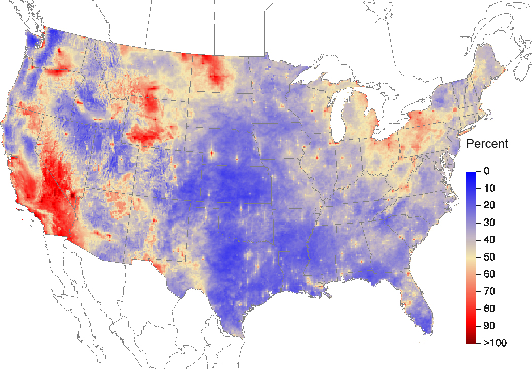
Figure 10-1 shows a map of TDep method estimates of dry deposition rates of sulfur (S) for 2016. Estimated rates of total deposition of sulfur for 2016 are given in Figure 10-2. The magnitude of the deposition fluxes is illustrated by the shading in the figure legends. The percentage of total deposition of S due to dry deposition is shown in Figure 10-3.
Deposition of Base Cations and Chloride
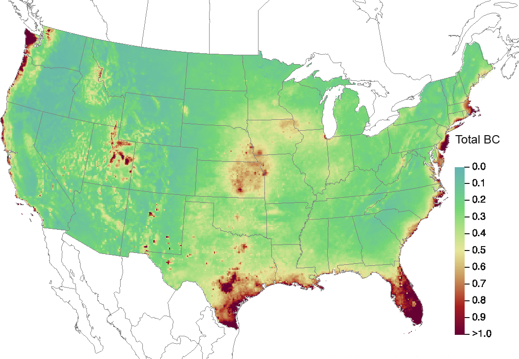
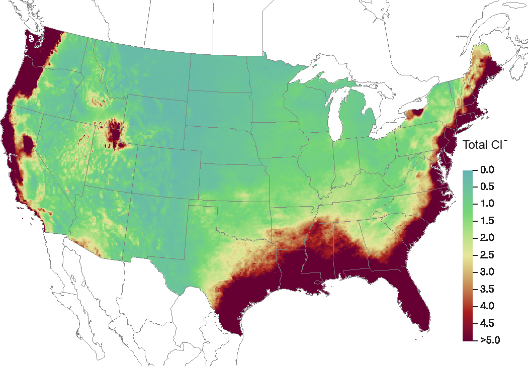
A map of 2016 estimated total deposition of base cations (Ca 2+ , K + , Mg 2+ , and Na + ) is given in Figure 10-4. Figure 10-5 provides estimated rates for 2016 for total deposition of Cl -.
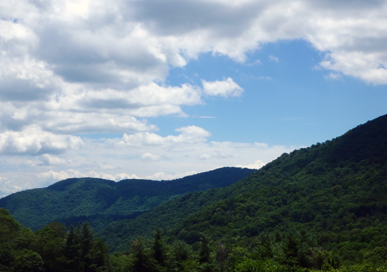
Scenic View from PNF126, NC
Figure 10-1 TDep Dry Deposition Estimates of S (kg ha -1 yr -1) for 2016
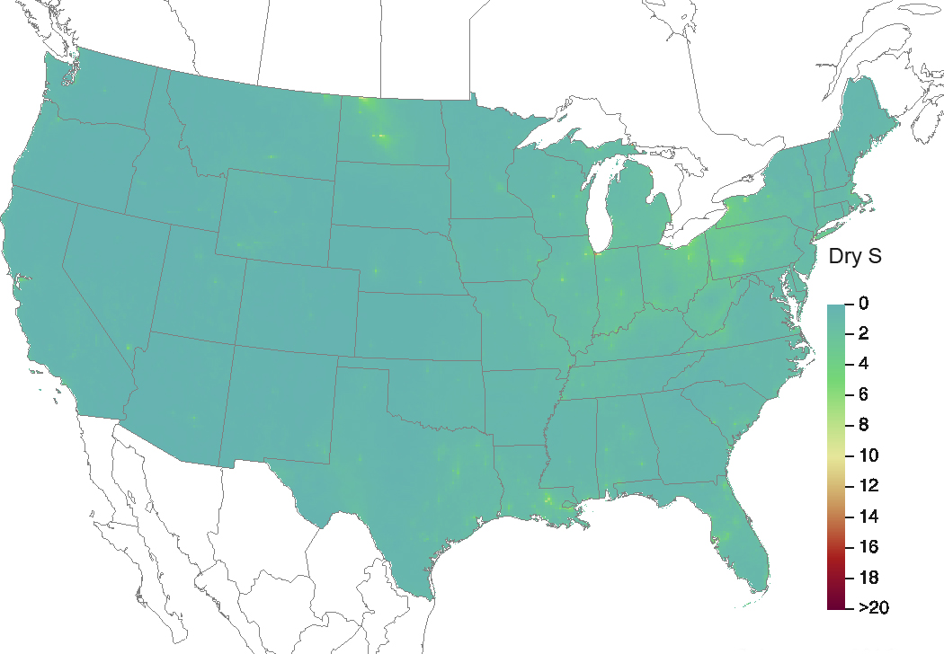
Source: CASTNET|CMAQ|NADP/NTN
Download FigureFigure 10-2 TDep Total Deposition Estimates of S (kg ha -1 yr -1) for 2016
Source: CASTNET|CMAQ|NADP/NTN
Download FigureFigure 10-3 TDep Percent of Total Deposition of S from Dry Deposition for 2016
Source: CASTNET|CMAQ|NADP/NTN
Download FigureFigure 10-4 TDep Total Deposition Estimates of the Base Cations Ca 2+ , K + , Mg 2+, Na + (kiloequivalents per hectare per year) for 2016
Source: CASTNET|CMAQ|NADP/NTN
Download FigureFigure 10-5 TDep Total Deposition Estimates of Total Cl - (kg ha -1 yr -1) for 2016
Source: CASTNET|CMAQ|NADP/NTN
Download FigureChapter 11: Critical Loads for Open and Closed Canopy Herbaceous Ecosystems
Critical loads were estimated for biodiverse open and closed canopy herbaceous ecosystems based on TDep estimates of wet and dry deposition of nitrogen across the United States. Three-year averages for 2013–2015 were compared for the open and closed ecosystems. Open canopy systems had more extensive critical load exceedance rates than the closed systems. The analysis suggests that, for the majority of regions where data were available, the loss of herbaceous biodiversity due to air pollutant deposition is unlikely. However, areas in Minnesota and North Carolina are likely experiencing loss of herbaceous biodiversity because of elevated levels of nitrogen deposition.
Critical loads describe the threshold at which a natural system is impacted by deposition of nitrogen (N) and/or sulfur (S) air pollutants. Critical loads provide tools that allow the evaluation of the sensitivity and the potential impact of air pollution on terrestrial and aquatic ecosystems. This chapter focuses on critical loads for herbaceous biodiversity and their potential exceedances. A critical load exceedance is the case when deposition is greater than the critical load (e.g., total deposition of N > critical load). Critical load exceedances indicate (1) a risk of negative impacts to natural resources as a result of air pollutant deposition, (2) whether pollutant deposition might be impacting natural systems, and (3) where impacts to the landscape might be occurring. For ecosystems impacted by deposition of pollutants, changes in critical load exceedances provide information to indicate if deposition has improved enough to allow ecosystem recovery, to judge the effectiveness of emission reduction policies and strategies, and to inform land management decisions.
The critical loads for herbaceous biodiversity were determined by Simkin et al. (2016) and were based on total deposition of N (wet and dry). The critical loads describe the level of deposition of N above which decreases in herbaceous plant species richness (i.e., total number of unique species per plot of land) were observed. They are expressed in terms of kg ha -1 yr -1 of N deposition. The analysis by Simkin et al. (2016) used a nationwide statistical analysis of 15,136 forest, woodland, shrubland, and grassland sites assembled from 12 distinct data sets.
The critical loads from Simkin et al. (2016) were calculated separately for open canopy and closed canopy systems based on Level 1 of the U. S. National Vegetation Classification (USNVC, 2016). A total of 11,819 plots were located in closed canopy systems while 3,317 were in open canopy systems. An open system includes grasslands, shrublands, and woodlands. A closed system includes those herbaceous species growing in the forest understories. This distinction was made because reduced sunlight limits the growth, reproduction, and other biological factors that in turn reduce the richness of the herbaceous community growing in the understory of forests (Neufeld and Young, 2014).
Critical loads were derived statistically using multiple regression models relating the species richness of a plot to environmental factors that included deposition of N, temperature, precipitation, soil pH, and others. A critical load was then estimated using a two-step process whereby the partial derivative of the best statistical model was selected, which yielded an equation for the critical load based on temperature, precipitation, and soil pH. Using that equation, the critical load was calculated at a given plot using local environmental data.
Critical load exceedances were evaluated using total N deposition values derived from TDep simulations (Chapter 8). A three-year average from 2013–2015 was compared to each plot for both open and closed systems. The range of the critical loads for closed canopy forest was 7.3 to 19.6 kg ha -1 yr -1 of N deposition, while open canopy environments were lower with a range of 7.4 to 9.0 kg ha -1 yr -1 of N deposition (Figure 11-1). Open canopy sites are designated as triangles while closed canopy systems are noted as circles. Figure 11-2 shows the spatial extent of critical load exceedances where data were available. Green triangles/circles show sites where the critical load was not exceeded while red triangles/circles indicate deposition greater than the critical load. Yellow triangles/circles show the sites where deposition of N was within 1 kg ha -1 yr -1 of the critical load. The open canopy systems had a higher exceedance rate (red triangles) of 22.7 percent than the closed canopy systems of 1.6 percent (red circles). The regions with the higher exceedances are in Minnesota and North Carolina. There were also many examples where deposition was near (i.e., within 1 kg ha -1 yr -1 ) the critical load (yellow circles/triangles) for closed and open systems. Sites that did not exceed the critical load were far more common. Open canopy sites did not exceed their critical load 69 percent of the time (green triangles) while forested systems did not exceed their critical load at 94 percent of the sites (green circles). This analysis suggests that, for the majority of regions where data were available, the loss of herbaceous biodiversity due to air pollution is unlikely. However, areas in Minnesota and North Carolina are likely experiencing loss of herbaceous biodiversity because of the deposition of elevated levels of N to these systems.
Figure 11-1 Critical Loads of Nitrogen Deposition for Herbaceous Biodiverse Ecosystems Determined by Simkin et al. (2016)
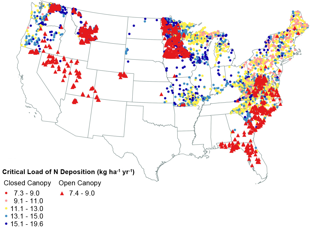 Download Figure
Figure 11-2 Critical Loads Exceedance for Herbaceous Biodiverse Ecosystems from TDep Deposition Estimates
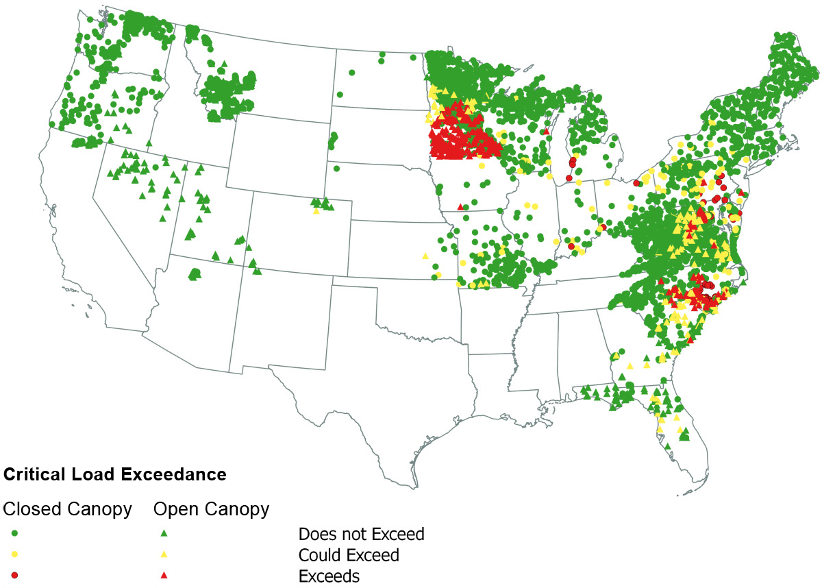 Download Figure
References
Air Resource Specialists (ARS). 2015. Gaseous Pollutant Monitoring Program Quality Assurance Project Plan (QAPP) Revision 3. Prepared for the National Park Service, Air Resources Division, Denver, CO. https://www.nature.nps.gov/air/Monitoring/docs/2010510_NPS_ARD_GPMP_QAPP.pdf Accessed May 2018.
Atmospheric Sciences Research Center (ASRC). 2017. Air Quality Monitoring. http://pireds.asrc.cestm.albany.edu:3000/. Accessed June 2018.
Baumann, K., Williams, E. J., Olson, J. A., Harder, J. W., and Fehsenfeld F. C. 1997. Meteorological Characteristics and Spatial Extent of Upslope Events during the 1993 Tropospheric OH Photochemistry Experiment. J. Geophys. Res., 102(D5), 6199–6213, doi: 10.1029/96JD03251.
Byun, D. and Schere, K. L. 2006. Review of the Governing Equations, Computational Algorithms, and Other Components of the Models‐3 Community Multiscale Air Quality (CMAQ) Modeling System. Applied Mechanics Reviews, 59: 51‐77. doi: 10.1115/1.2128636.
International Organization for Standardization (ISO). 2005. Statistical Methods for the Use in Proficiency Testing by Interlaboratory Comparisons, Annex C, Robust Analysis, Section C.1: Algorithm A. Standard 13528. ISO 13528:2005(E).
Lefohn, A. S. and Runeckles, V. C. 1987. Establishing a Standard to Protect Vegetation - Ozone Exposure/Dose Considerations. Atmos. Environ., 21:561-568.
Liu, X., Huey, L. G., Yokelson, R. J., Selimovic, V., Simpson, I. J., Muller, M., Jimenez, J. L., Campuzano-Jost, P., Beyersdorf, A. J., Blake, D. R., Butterfield, Z., Choi, Y., Crounse, J. D., Day, D. A., Diskin, G. S., Dubey, M. K., Fortner, E., Hanisco, T. F., Hu, W., King, L. E., Kleinman, L., Meinardi, S., Mikoviny, T. Onasch, T. B., Palm, B. B., Peischl, J., Pollack, I. B., Ryerson, T. B., Sasche, G. W., Sedlacek, A. J., Shilling, J. E., Springston, S., St. Clair, J. M., Tanner, D. J., Teng, A. P., Wennberg, P. O., Wisthaler, A., and Wolfe, G. M. 2017. Airborne Measurements of Western U.S. Wildfire Emissions: Comparison with Prescribed Burning and Air Quality Implications. J. Geophys. Res. Atmos., 122, 6108–6129, doi: 10.1002/2016JD026315.
Lyman, S., Mansfield, M., Tran, H., and Tran, T. 2016. Annual Report. Uintah Basin Air Quality Research Project. Utah State University. Prepared for Utah Legislature, Document Number: BRC_161116A.
Martin, R. S. and Baasandorj, M. 2016. A Comparison of AMoN Measurements with Localized, Arrayed Passive NH3 Samplers in Northern Utah. National Atmospheric Deposition Program (NADP), 2016 Fall Meeting, Santa Fe, NM, Oct. 31–Nov. 4.
National Aeronautic and Space Administration (NASA). 2016. NASA Satellite Sees Smoke Streaming from Arizona's Jack Fire. Land Atmosphere Near Real-time Capability (LANCE)/Earth Observing System Data and Information System (EOSDIS) Moderate Resolution Imaging Spectroradiometer (MODIS) Rapid Response Team, Goddard Space Flight Center (GSFC) https://www.nasa.gov/image-feature/goddard/2016/nasa-satellite-sees-smoke-streaming-from- arizonas-jack-fire. Accessed November 2017.
National Oceanic and Atmospheric Administration (NOAA)/National Aeronautic and Space Administration (NASA). 2016. Maple Fire Threatens Western Edge of Yellowstone National Park. Environmental Visualization Laboratory. https://www.nasa.gov/image- feature/goddard/2016/maple-fire-threatens-western-edge-of-yellowstone-national-park. Accessed November 2017.
National Oceanic and Atmospheric Administration (NOAA) National Centers for Environmental Prediction (NCEP), Weather Prediction Center. 2016. Daily Weather Map, June 14 and June 17, 2016. https://www.wpc.ncep.noaa.gov/dailywxmap/index_20160614.html and https://www.wpc.ncep.noaa.gov/dailywxmap/index_20160617.html. Accessed August 2018.
Neeman, E. M., Crosman, E. T., Horel, J. D., and Avey, L. 2015. Simulations of Cold-Air Pool Associated with Elevated Wintertime Ozone in the Uintah Basin, Utah. 2015. Atmos. Chem. Phys., 15, 135-151, 2015.
Neufeld, H., and Young. D. R. 2014. “Ecophysiology of the Herbaceous Layer in Temperate Deciduous Forests.” In Ecophysiology of the Herbaceous Layer in Forests of Eastern North America, edited by F. Gilliam, pp. 34–95. Oxford University Press, New York. doi: 10.1093/acprof:osobl/9780199837656.001.0001
Schwede, D. B. and Lear, G. G. 2014. A Novel Hybrid Approach for Estimating Total Deposition in the United States. Atmos. Environ., 92:207-220. doi: 10.1016/j.atmosenv.2014.04.008.
Schwede, D. B. and Lear, G. G. 2014. A Novel Hybrid Approach for Estimating Total Deposition in the United States. Atmos. Environ., 92:207-220. doi: 10.1016/j.atmosenv.2014.04.008.
Simkin, S. M., Allen, E. B., Bowman, W. D., Clark, C. M., Belnap, J., Brooks, M. L., Cade, B. S., Collins, S. L., Geiser, L. H., Gilliam, F. S., Jovan, S. E., Pardo, L. H., Schulz, B. K., Stevens, C. J. Suding, K. N., Throopo, H. L., and Waller, D. M. 2016. Conditional Vulnerability of Plant Diversity to Atmospheric Nitrogen Deposition across the United States. Proceedings of the National Academy of Sciences 113:4086-4091. doi: 10.1073/pnas.1515241113.
Talbot, R., Mao, H., and Sive, B. 2005. Diurnal Characteristics of Surface Level O3 and other Important Trace Gases in New England, J. Geophys. Res., 110, D09307, doi:10.1029/2004JD005449.
U.S. Environmental Protection Agency (EPA). 2017. Air Markets Program Data. https://ampd.epa.gov/ampd/ Accessed June 2018.
U.S. Environmental Protection Agency (EPA). 2016. Treatment of Air Quality Data Influenced by Exceptional Events. https://www.epa.gov/air-quality-analysis/treatment-air-quality-datainfluenced-exceptional-events. June 2018.
U.S. Environmental Protection Agency (EPA). 2015a. Clean Air Status and Trends Network Factsheet-2015. https://www3.epa.gov/castnet/docs/CASTNET-Factsheet-2015.pdf. Accessed May 2018.
U.S. Environmental Protection Agency (EPA). 2015b. Interpretation of the Primary and Secondary National Ambient Air Quality Standards for Ozone. Title 40 Code of Federal Regulations (CFR) Appendix U to Part 50. https://www.ecfr.gov/cgi-bin/ extidx?SID=9b5c394e6ac7be772c8f605a6554e08b&mc=true&node=pt40.2.50&rgn=div5#ap40.2.50_119.u. Accessed June 2018.
U.S. Environmental Protection Agency (EPA). 2015c. Title 40 Code of Federal Regulations (CFR) Part 50, Primary and Secondary National Ambient Air Quality Standards. https://www.ecfr.gov/cgi-bin/textidx?SID=b67492f51b28e27bf9b4226033416c93&mc=true&node=pt40.2.50&rgn=div5. Accessed June 2018.
U.S. Environmental Protection Agency (EPA). 2015d. Total Deposition Estimates Using a Hybrid Approach. ftp://ftp.epa.gov/castnet/tdep/Total_Deposition_Documentation_current.pdf. Accessed June 2018.
U.S. Environmental Protection Agency (EPA). 2014. National Emissions Inventory (NEI) Data. https://www.epa.gov/air-emissions-inventories/2014-national-emissions-inventory-nei-data Accessed March 27, 2017.
U.S. Environmental Protection Agency (EPA). 2008. National Ambient Air Quality Standards for Ozone; Final Rule. Federal Register 73, No. 60 (March). EPA-HQ-OAR-2005-0172.
U.S. National Vegetation Classification (USNVC). 2016. United States National Vegetation Classification Database, V2.0. Federal Geographic Data Committee, Vegetation Subcommittee, Washington DC. usnvc.org.
Ute Indian Tribe. 2016. Ozone NAAQS Exceedances Occurring June 8 and 9, 2015, Uinta Basin of Utah. Submitted to U.S. Environmental Protection Agency (EPA), Region 8, August 30, 2016.
Wood Environment & Infrastructure Solutions, Inc. (Wood)* . 2017a. Clean Air Status and Trends Network (CASTNET) Fourth Quarter 2016 Data Report. Prepared for U.S. Environmental Protection Agency (EPA), Office of Air and Radiation, Clean Air Markets Division, Washington, DC. Contract No. EP-W-15-003. Gainesville, FL.
Wood Environment & Infrastructure Solutions, Inc. (Wood)* . 2017b. Clean Air Status and Trends Network (CASTNET) Third Quarter 2016 Data Report. Prepared for U.S. Environmental Protection Agency (EPA), Office of Air and Radiation, Clean Air Markets Division, Washington, DC. Contract No. EP-W-15-003. Gainesville, FL.
Wood Environment & Infrastructure Solutions, Inc. (Wood)* . 2016a. Clean Air Status and Trends Network (CASTNET) First Quarter 2016 Data Report. Prepared for U.S. Environmental Protection Agency (EPA), Office of Air and Radiation, Clean Air Markets Division, Washington, DC. Contract No. EP-W-15-003. Gainesville, FL.
Wood Environment & Infrastructure Solutions, Inc. (Wood)* . 2016b. Clean Air Status and Trends Network (CASTNET) Second Quarter 2016 Data Report. Prepared for U.S. Environmental Protection Agency (EPA), Office of Air and Radiation, Clean Air Markets Division, Washington, DC. Contract No. EP-W-15-003. Gainesville, FL.
Wood Environment & Infrastructure Solutions, Inc. (Wood)*. 2015. Clean Air Status and Trends Network (CASTNET) Quality Assurance Project Plan (QAPP) Revision 8.3. Prepared for U.S. Environmental Protection Agency (EPA), Office of Air and Radiation, Clean Air Markets Division, Washington, DC. Contract No. EP-W-09-028. Gainesville, FL. http://java.epa.gov/castnet/documents.do.
Wood Environment & Infrastructure Solutions, Inc. (Wood)*. 2012. Clean Air Status and Trends Network (CASTNET) 2010 Annual Report. Prepared for U.S. Environmental Protection Agency (EPA), Office of Air and Radiation, Clean Air Markets Division, Washington, DC. Contract No. EP-W-09-028. Gainesville, FL.
Youden, W.J. (Ku, H.H., ed). 1969. Precision Measurement and Calibration. NBS Special Publication 300-Volume 1. U.S. Government Printing Office, Washington, DC.
* Formerly known as Amec Foster Wheeler Environment & Infrastructure, Inc.
Appendix A: Locational and Operational Characteristics of CASTNET Sites
| Site ID | Site Name | Start date | Latitude | Longitude | Elevation | Nearby NADP |
Land Use |
Terrain | Agency | Reference |
|---|---|---|---|---|---|---|---|---|---|---|
| ABT147, CT | Abington | 12/28/1993 | 41.8405 | -72.0104 | 202 | CT15 | Urban/ Agric |
Rolling | EPA | |
| ACA416, ME | Acadia NP | 12/1/1998 | 44.3771 | -68.2608 | 158 | ME98 | Forest | Rolling | NPS | |
| ALC188, TX | Alabama- Coushatta |
4/6/2004 | 30.7016 | -94.674 | 105 | TX10 | Prairie | Rolling | EPA | |
| ALH157, IL | Alhambra | 6/28/1988 | 38.869 | -89.6228 | 164 | IL46 | Agric | Flat | EPA | E |
| ANA115, MI | Ann Arbor | 6/28/1988 | 42.4166 | -83.9022 | 266 | MI52 | Forest | Flat | EPA | E |
| ARE128, PA | Arendtsville | 6/28/1988 | 39.9232 | -77.3079 | 266 | PA00 | Agric | Rolling | EPA | E |
| ASH135, ME | Ashland | 12/20/1988 | 46.6038 | -68.4132 | 231 | ME00 | Agric | Flat | EPA | E |
| BAS601, WY | Basin | 11/6/2012 | 44.28 | -108.0411 | 1242 | MT00 | Prairie | Rolling | BLM | |
| BBE401, TX | Big Bend NP | 7/18/1995 | 29.3027 | -103.1778 | 1052 | TX04 | Forest | Complex | NPS | W |
| BEL116, MD | Beltsville | 11/1/1988 | 39.0282 | -76.8171 | 47 | MD99 | Range | Flat | EPA | E |
| BFT142, NC | Beaufort | 12/28/1993 | 34.8847 | -76.6207 | 5 | NC06 | Agric | Flat | EPA | |
| BUF603, WY | Buffalo | 11/6/2012 | 44.1442 | -106.1089 | 1324 | WY99 | Prairie | Rolling | BLM | |
| BVL130, IL | Bondville | 2/9/1988 | 40.052 | -88.3725 | 213 | IL11 | Agric | Flat | EPA | E |
| BWR139, MD | Blackwater NWR |
7/4/1995 | 38.445 | -76.1113 | 1 | MD15 | Forest/ Marsh |
Coastal | EPA | |
| CAD150, AR | Caddo Valley |
10/4/1988 | 34.1793 | -93.0988 | 78 | AR03 | Forest | Complex | EPA | E |
| CAN407, UT | Canyonlands NP |
1/24/1995 | 38.4583 | -109.8213 | 1809 | UT09 | Desert | Complex | NPS | W |
| CAT175, NY | Claryville | 5/10/1994 | 41.9423 | -74.552 | 754 | NY68 | Forest | Complex | EPA | |
| CDR119, WV | Cedar Creek | 11/10/1987 | 38.8795 | -80.8477 | 240 | WV05 | Forest | Complex | EPA | E |
| CDZ171, KY | Cadiz | 1/5/1999 | 36.7841 | -87.8502 | 190 | KY99 | Agric | Rolling | EPA | |
| CHA467, AZ | Chiricahua NM |
4/25/1989 | 32.0094 | -109.3891 | 1570 | AZ98 | Range | Complex | NPS | W |
| CHE185, OK | Cherokee Nation |
4/2/2002 | 35.7508 | -94.6698 | 305 | AR27 | Agric | Rolling | EPA | |
| CKT136, KY | Crockett | 8/24/1993 | 37.9215 | -83.0663 | 376 | KY35 | Agric | Rolling | EPA | |
| CND125, NC | Candor | 9/25/1990 | 35.2633 | -79.8375 | 172 | NC36 | Forest | Rolling | EPA | E |
| CNT169, WY | Centennial | 5/9/1989 | 41.3645 | -106.24 | 3175 | WY95 | Forest | Complex | EPA | W |
| COW005, NC | Coweeta Screwdriver Knob |
11/18/2014 | 35.0469 | -83.4531 | 960 | NC25 | Forest | Complex | EPA | |
| COW137, NC | Coweeta | 11/4/1987 | 35.0605 | -83.4303 | 683 | NC25 | Forest | Complex | EPA | E |
| CTH110, NY | Connecticut Hill |
9/29/1987 | 42.4009 | -76.6535 | 511 | NY67 | Forest | Rolling | EPA | E |
| CVL151, MS | Coffeeville | 12/27/1988 | 34.0027 | -89.7992 | 138 | MS30 | Forest | Rolling | EPA | |
| DCP114, OH | Deer Creek | 9/28/1988 | 39.6359 | -83.2606 | 264 | OH54 | Agric | Rolling | EPA | E |
| DEN417, AK | Denali NP | 10/6/1998 | 63.7232 | -148.9676 | 661 | AK03 | Forest | Complex | NPS | |
| DIN431, UT | Dinosaur NM | 11/20/2013 | 40.4373 | -109.3046 | 1463 | CO15 | Desert | Complex | NPS | |
| EGB181, ON | Egbert | 12/27/1994 | 44.2311 | -79.7831 | 227 | NY10 | Agric | Rolling | EPA | |
| ESP127, TN | Edgar Evins | 3/22/1988 | 36.0389 | -85.7331 | 302 | KY10 | Forest | Rolling | EPA | E |
| EVE419, FL | Everglades NP |
10/6/1998 | 25.3912 | -80.6808 | 2 | FL11 | Forest/ Marsh |
Flat | NPS | |
| FOR605, WY | Fortification Creek |
5/21/2013 | 44.3395 | -105.9198 | 1408 | WY99 | Prairie | Rolling | BLM | |
| GAS153, GA | Georgia Station |
6/28/1988 | 33.1812 | -84.4101 | 265 | GA41 | Agric | Rolling | EPA | E |
| GLR468, MT | Glacier NP | 12/27/1988 | 48.5103 | -113.9968 | 976 | MT05 | Forest | Complex | NPS | W |
| GRB411, NV | Great Basin NP |
5/16/1995 | 39.0051 | -114.2159 | 2060 | NV05 | Forest | Complex | NPS | W |
| GRC474, AZ | Grand Canyon NP |
5/16/1989 | 36.0586 | -112.1836 | 2073 | AZ03 | Forest | Rolling | NPS | W |
| GRS420, TN | Great Smoky NP- Look Rock |
10/16/1998 | 35.6335 | -83.9416 | 793 | TN11 | Forest | Complex | NPS | |
| GTH161, CO | Gothic | 5/16/1989 | 38.9563 | -106.9859 | 2915 | CO10 | Range | Complex | EPA | W |
| HOW191, ME | Howland Ameriflux |
9/27/2011 | 45.204 | -68.74 | 68 | ME09 | Forest | Rolling | EPA | |
| HOX148, MI | Hoxeyville | 10/31/2000 | 44.1809 | -85.739 | 297 | MI53 | Forest | Flat | EPA | |
| HWF187, NY | Huntington Wildlife Forest |
5/28/2002 | 43.973 | -74.2233 | 497 | NY20 | Forest | Complex | EPA | |
| IRL141, FL | Indian River Lagoon |
7/9/2001 | 27.8492 | -80.4556 | 2 | FL99 | Coastal/ Marsh | Flat/ Water | EPA | |
| JOT403, CA | Joshua Tree NP |
2/16/1995 | 34.0696 | -116.3889 | 1244 | CA67 | Desert | Complex | NPS | W |
| KEF112, PA | Kane Experimental Forest |
1/3/1989 | 41.5981 | -78.7679 | 618 | PA29 | Forest | Rolling | EPA | E |
| KIC003, KS | Kickapoo Tribe |
2/18/2014 | 39.8539 | -95.6578 | 367 | KS97 | Prairie | Rolling | EPA | |
| KNZ184, KS | Konza Prairie |
3/26/2002 | 39.1022 | -96.6096 | 346 | KS31 | Prairie | Flat | EPA | |
| LAV410, CA | Lassen Volcanic NP |
7/25/1995 | 40.54 | -121.5765 | 1756 | CA96 | Forest | Complex | NPS | W |
| LRL117, PA | Laurel Hill | 12/15/1987 | 39.9883 | -79.2516 | 609 | PA83 | Forest | Complex | EPA | E |
| MAC426, KY | Mammoth Cave NP |
7/24/2002 | 37.1314 | -86.1481 | 243 | KY10 | Agric | Rolling | NPS | |
| MCK131, KY | Mackville | 7/31/1990 | 37.7047 | -85.0487 | 293 | KY03 | Agric | Rolling | EPA | E |
| MCK231, KY | Mackville Co-located |
12/29/1992 | 37.7047 | -85.0487 | 293 | KY03 | Agric | Rolling | EPA | |
| MEV405, CO | Mesa Verde NP | 1/10/1995 | 37.1984 | -108.4905 | 2165 | CO99 | Forest | Complex | NPS | W |
| MKG113, PA | M.K. Goddard | 1/12/1988 | 41.4268 | -80.1452 | 377 | NY10 | Forest | Rolling | EPA | E |
| NEC602, WY | Newcastle | 11/7/2012 | 43.873 | -104.1919 | 1468 | WY99 | Prairie | Rolling | BLM | |
| NIC001, NY | Nicks Lake | 11/20/2012 | 43.6805 | -74.9891 | 525 | NY29 | Forest | Rolling | NYSDEC | |
| NPT006, ID | Nez Perce Tribe |
12/15/2015 | 46.2756 | -116.0216 | 945 | Forest | Rolling | EPA | ||
| OXF122, OH | Oxford | 8/18/1987 | 39.5311 | -84.7235 | 284 | OH09 | Agric | Rolling | EPA | E |
| PAL190, TX | Palo Duro SP | 4/24/2007 | 34.8806 | -101.6647 | 1053 | TX02 | Prairie | Complex | EPA | |
| PAR107, WV | Parsons | 1/19/1988 | 39.0904 | -79.6617 | 510 | WV18 | Forest | Complex | EPA | E |
| PED108, VA | Prince Edward |
11/3/1987 | 37.1652 | -78.3071 | 149 | VA24 | Forest | Rolling | EPA | E |
| PET427, AZ | Petrified Forest |
9/12/2002 | 34.8225 | -109.8925 | 1723 | AZ97 | Desert | Flat | NPS | |
| PIN414, CA | Pinnacles NM | 5/16/1995 | 36.4832 | -121.1569 | 335 | CA66 | Forest | Complex | NPS | W |
| PND165, WY | Pinedale | 12/27/1988 | 42.929 | -109.7878 | 2386 | WY06 | Forest | Rolling | EPA | W |
| PNF126, NC | Cranberry | 12/27/1988 | 36.1054 | -82.045 | 1216 | NC45 | Forest | Mountain-top | EPA | E |
| PRK134, WI | Perkinstown | 9/27/1988 | 45.2065 | -90.5972 | 462 | WI35 | Agric | Rolling | EPA | E |
| PSU106, PA | Penn State | 1/6/1987 | 40.7209 | -77.9318 | 364 | PA42 | Agric | Rolling | EPA | E |
| QAK172, OH | Quaker City | 1/5/1999 | 39.9427 | -81.3379 | 371 | OH49 | Agric | Rolling | EPA | |
| RED004, MN | Red Lake Nation |
8/26/2014 | 47.8638 | -94.8352 | 372 | MN16 | Forest | Flat | EPA | |
| ROM206, CO | Rocky Mountain NP Co-located |
7/3/2001 | 40.2781 | -105.5456 | 2742 | CO19 | Forest | Complex | EPA | |
| ROM406, CO | Rocky Mountain NP |
12/20/1994 | 40.2781 | -105.5456 | 2743 | CO19 | Forest | Complex | NPS | W |
| SAL133, IN | Salamonie Reservoir |
6/28/1988 | 40.816 | -85.6614 | 250 | IN20 | Agric | Flat | EPA | E |
| SAN189, NE | Santee Sioux | 7/5/2006 | 42.8292 | -97.8541 | 434 | SD99 | Range | Rolling | EPA | |
| SEK430, CA | Sequoia & Kings Canyon NP - Ash Mountain |
4/7/2005 | 36.4895 | -118.8292 | 510 | CA75 | Forest | Mountain- top | NPS | |
| SHE604, WY | Sheridan | 11/6/2012 | 44.93 | -106.85 | 1115 | MT00 | Prairie | Rolling | BLM | |
| SHN418, VA | Shenandoah NP- Big Meadows |
6/28/1988 | 38.5231 | -78.4347 | 1073 | VA28 | Forest | Mountain- top | NPS | E |
| SND152, AL | Sand Mountain | 12/27/1988 | 34.289 | -85.9701 | 349 | AL99 | Agric | Rolling | EPA | E |
| SPD111, TN | Speedwell | 6/12/1989 | 36.4698 | -83.8265 | 361 | TN04 | Agric | Rolling | EPA | E |
| STK138, IL | Stockton | 12/28/1993 | 42.2872 | -90 | 281 | IL18 | Agric | Rolling | EPA | |
| SUM156, FL | Sumatra | 12/27/1988 | 30.1102 | -84.9904 | 16 | FL23 | Forest | Flat | EPA | E |
| THR422, ND | Theodore Roosevelt NP |
10/6/1998 | 46.8948 | -103.3777 | 850 | ND00 | Forest | Rolling | NPS | |
| UND002, VT | Underhill | 11/13/2012 | 44.5283 | -72.8688 | 399 | VT99 | Forest | Complex | EPA | |
| UVL124, MI | Unionville | 6/28/1988 | 43.6136 | -83.3599 | 202 | MI51 | Agric | Flat | EPA | E |
| VIN140, IN | Vincennes | 8/4/1987 | 38.7408 | -87.4849 | 136 | IN22 | Agric | Rolling | EPA | E |
| VOY413, MN | Voyageurs NP | 6/13/1996 | 48.4125 | -92.8292 | 429 | MN32 | Forest | Rolling | NPS | |
| VPI120, VA | Horton Station | 6/2/1987 | 37.3298 | -80.5575 | 920 | VA13 | Agric | Mountain- top | EPA | E |
| WFM007, NY | Whiteface Mountain Summit |
6/4/2015 | 44.36608 | -73.90312 | 1415 | NY98 | Forest | Complex | EPA | |
| WFM105, NY | Whiteface Mountain |
11/20/2012 | 44.39 | -73.86 | 570 | NY98 | Forest | Complex | NYSDEC | |
| WNC429, SD | Wind Cave NP | 11/20/2003 | 43.5576 | -103.4839 | 1292 | SD04 | Prairie | Rolling | NPS | |
| WSP144, NJ | Washington Crossing |
12/27/1988 | 40.3123 | -74.8727 | 59 | NJ99 | Range | Rolling | EPA | E |
| WST109, NH | Woodstock | 12/27/1988 | 43.9445 | -71.7008 | 255 | NH02 | Forest | Complex | EPA | E |
| YEL408, WY | Yellowstone NP | 6/26/1996 | 44.5654 | -110.4003 | 2400 | WY08 | Agric | Rolling | NPS | W |
| YOS404, CA | Yosemite NP - Turtleback Dome |
9/25/1995 | 37.7133 | -119.7062 | 1605 | CA99 | Forest | Complex | NPS | W |
Note:
NM = National Monument
NP = National Park
NWR = National Wildlife Reserve
SP = State Park
E = eastern reference site
W = western reference site
Appendix B: Acronyms and Abbreviations
| A2LA | American Association for Laboratory Accreditation |
| Amec Foster Wheeler | Amec Foster Wheeler Environment & Infrastructure, Inc. |
| AMNet | Atmospheric Mercury Network |
| AMoN | Ammonia Monitoring Network |
| AQS | EPA's Air Quality System |
| ARP | Acid Rain Program |
| ASRC | Atmospheric Sciences Research Center |
| BLM | Bureau of Land Management |
| C-R | concentation-response |
| Ca | particulate calcium |
| CAAA | Clean Air Act Amendments |
| CAMx | Comprehensive Air Quality Model with Extensions |
| CAPMoN | Canadian Air and Precipitation Monitoring Network |
| CASTNET | Clean Air Status and Trends Network |
| CFR | Code of Federal Regulations |
| Cl - | particulate chloride |
| CMAQ | Community Multiscale Air Quality Modeling System |
| CO | carbon monoxide |
| CSAPR | Cross-State Air Pollution Rule |
| DM8A | daily maximum 8-hour average |
| DQI | data quality indicator |
| ECAN | Environment Canada |
| EGUs | electric generating units |
| EPA | U.S. Environmental Protection Agency |
| Hg | mercury |
| HNO | nitric acid |
| HONO | nitrous acid |
| HYSPLIT | Hybrid Single Particle Lagrangian Integrated Trajectory model |
| IEC | International Electrotechnical Commission |
| IMPROVE | Interagency Monitoring of Protected Visual Environments |
| ISO | International Organization for Standardization |
| K | particulate potassium |
| kg ha yr | kilograms per hectare per year |
| km | kilometer |
| m | meter |
| MADPro | Mountain Acid Deposition Program |
| MARGA | Monitor for Aerosols and Gases in Ambient Air |
| MARPD | mean absolute relative percent difference |
| MCCP | Mountain Cloud Chemistry Project |
| MDL | method detection limit |
| MDN | Mercury Deposition Network |
| Mg | particulate magnesium |
| mg/L | milligrams per liter |
| MRPD | mean relative percent difference |
| MU | MARGA unit |
| N | nitrogen |
| Na | particulate sodium |
| NAAQS | National Ambient Air Quality Standards |
| NADP | National Atmospheric Deposition Program |
| NAPAP | National Acid Precipitation and Assessment Program |
| NCore | EPA's National Core Monitoring |
| NH | ammonia |
| NH | particulate ammonium |
| NHNO | ammonium nitrate |
| NO | nitrogen oxide |
| NO | nitrogen dioxide |
| NO | particulate nitrate |
| NOx | nitrogen oxides [nitrogen oxide (NO) + nitrogen dioxide (NO)] |
| NOy | total reactive oxides of nitrogen |
| NOz | HNO, nitrous oxide, peroxyacetyl nitrate, peroxyproyl nitrate, other organic nitrates, and nitrite |
| NPS | National Park Service |
| NTN | National Trends Network |
| NYSDEC | New York State Department of Environmental Conservation |
| O | ozone |
| PFA | pulsed fluorescence analyzer |
| PM | particulate matter |
| PM2.5 | fine particulate matter |
| ppb | parts per billion |
| ppm | parts per million |
| PRISM | Parameter-elevation Regressions on Independent Slopes Model |
| PT | proficiency testing |
| QA | quality assurance |
| QAPP | Quality Assurance Project Plan |
| QC | quality control |
| R2 | coefficient of determination |
| S | sulfur |
| SCR | selective catalytic reduction |
| SEARCH | Southeastern Aerosol Research and Characterization Network |
| SO | sulfur dioxide |
| SO | particulate sulfate |
| TDEP | NADP Total Deposition Hybrid Method |
| total NO | gaseous nitric acid (HNO) + particulate nitrate (NO) |
| TSP | total suspended particles |
| USDA | U.S. Department of Agriculture |
| µeq/L | microequivalents per liter |
| µg/m | micrograms per cubic meter |
| WARMS | Wyoming Air Resources Monitoring System |