Executive Summary
The EPA Clean Air Status and Trends Network (CASTNET) measures concentrations of atmospheric pollutants across the United States. The primary objectives of the network are to determine compliance with ozone National Ambient Air Quality Standards and to provide data to evaluate the effectiveness of national and regional air pollution control programs. CASTNET data are also used to provide input to the National Atmospheric Deposition Program’s Total Deposition Hybrid Method for calculating total deposition and evaluating regional air quality models. This report presents maps of 2015 ozone levels, nitrogen and sulfur pollutant concentrations, and deposition fluxes and examines trends in air quality over the 26-year period from 1990 through 2015. In 2015, CASTNET measured rural, regionally representative concentrations of nitrogen and sulfur species at 95 monitoring stations at 93 locations and ozone levels at 80 locations.
Key Results and Highlights through 2015
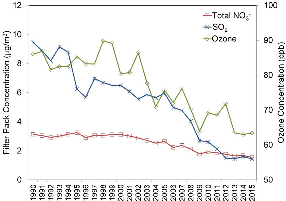
The median fourth highest daily maximum 8-hour average (DM8A) ozone (O3) concentration for 2015 at the eastern CASTNET reference sites (see Appendix A for designated reference sites) was 63.5 parts per billion (ppb) or, equivalently, 0.0635 parts per million (ppm). This is a slight increase from the 2014 median of 62.5 ppb, which was the lowest in the history of the network. At the western CASTNET reference sites, the median was 66 ppb. Three-year averages of fourth highest DM8A O3 concentrations exceeded the 2008 8-hour National Ambient Air Quality Standard (NAAQS) of 0.075 ppm at two California CASTNET sites during the most recent 3-year period (2013–2015). For 2015, the same two CASTNET sites in California measured fourth highest DM8A O3 concentrations greater than 0.075 ppm. Three-year averages of fourth highest DM8A O3 concentrations have been reduced by 25 percent at the eastern reference sites since 1990–1992 and by 9 percent at the western reference sites since 1996–1998. Figure E-1 and Table E-1 summarize the long-term changes in measured concentrations.
Regional O3 concentrations are influenced by nitrogen oxides (NOx) emissions. Federal, state, and local NOx control programs have resulted in substantive reductions in emissions. For example, NOx emissions declined by 79 percent over the 26 year period, 1990 through 2015, at regulated electric generating units (EGUs) in the East.
Three-year mean annual concentrations of total nitrate (NO3-), which is comprised of nitric acid (HNO3) plus particulate NO3-, declined 46 percent at the eastern reference sites over the 26-year period. Three-year mean annual total NO3- levels measured at the western reference sites dropped by 30 percent over the 20-year period.
Mean annual sulfur dioxide (SO2) concentrations measured at the eastern reference sites have declined significantly over the 26-year period, 1990 through 2015. Three-year mean annual SO2 levels at eastern sites decreased 83 percent. SO2 concentrations measured at the western reference sites declined by 47 percent over the 20 years from 1996 through 2015.
The percent reduction in SO2 concentrations at the eastern reference sites is consistent with the reduction in regulated eastern EGU SO2 emissions (86 percent).
Table E-1 Trends in Aggregated Western and Eastern O3, Total NO3-, and SO2 Pollutant Concentrations
| Pollutant | Western Sites | Eastern Sites | Percent Changed | |||
|---|---|---|---|---|---|---|
| 1996-98 | 2012-15 | 1990-92 | 2012-15 | West | East | |
| O3 (ppb) | 74 | 67 | 85 | 63 | -9 | -25 |
| Total NO3- (μg/m 3) | 1.0 | 0.7 | 3.0 | 1.6 | -30 | -46 |
| SO2 (μg/m 3) | 0.6 | 0.3 | 8.8 | 1.4 | -47 | -83 |
The original intent of CASTNET was to measure pollutant concentrations to estimate trends in sulfur and nitrogen pollutants. Currently, the focus also includes demonstrating compliance of rural, regional O3 concentrations with the NAAQS. The network also features measurements of trace-level gases and speciated nitrogen pollutants. Additionally, CASTNET supports the National Atmospheric Deposition Program’s Ammonia Monitoring Network with operation of ammonia samplers at 68 CASTNET sites. This report provides information on CASTNET pollutant measurements and estimated deposition fluxes and other topics such as forest health in the eastern United States and cloud water and filter pack pollutant concentrations measured on Whiteface Mountain, New York.
Chapter 1: CASTNET Update
The Clean Air Status and Trends Network (CASTNET) is a nationwide air quality monitoring network that has been operating for more than 25 years. The network performs long-term measurements of air pollutant concentrations in rural areas across the United States to determine compliance with ozone National Ambient Air Quality Standards and to evaluate the effectiveness of national and regional emission control programs. CASTNET was designed to identify trends in rural ozone, nitrogen, and sulfur concentrations and deposition rates of nitrogen and sulfur pollutants. CASTNET data are used for air quality program and strategy evaluation and to provide input for operation and evaluation of regional air quality models such as the National Atmospheric Deposition Program’s Total Deposition Hybrid Method. CASTNET is managed and operated by the U.S. Environmental Protection Agency in cooperation with the National Park Service and other federal, state, and local partners. In 2015, the network operated 95 monitoring stations throughout the contiguous United States, Alaska, and Canada. CASTNET data show a 26-year decline in ozone, nitrogen, and sulfur pollutant concentrations.
Introduction
The U.S. Congress established the Acid Rain Program (ARP) in 1990 under Title IV of the Clean Air Act Amendments (CAAA). The ARP was enacted to reduce emissions of sulfur dioxide (SO2) and nitrogen oxides (NOx) from electric generating units (EGUs) and has produced significant reductions in emissions since 1995. Since then, other air pollution control programs have been instituted to reduce emissions of SO2 and NOx. Examples of these control programs include the following:
- 1990 Ozone (O3) Transport Commission NOx Budget Program
- 1998 NOx State Implementation Plan Call
- 2003 NOx Budget Trading Program
- 2009 Clear Air Interstate Rule
- 2011 Cross-State Air Pollution Rule (CSAPR)
On January 1, 2015, implementation of the CSAPR Phase I began. The CSAPR was promulgated in 2011, requiring 28 states in the eastern half of the United States to significantly improve air quality by reducing EGU emissions that cross state lines and contribute to ground-level O3 and fine particulate matter (PM2.5) in downwind states. CSAPR was enacted under the Clean Air Act’s good neighbor provision to address regional interstate transport of O3 and PM2.5 pollution for the 1997 National Ambient Air Quality Standards (NAAQS) and the 2006 PM2.5 NAAQS. The rule requires reductions in annual SO2, annual NOx, and O3 season NOx emissions.
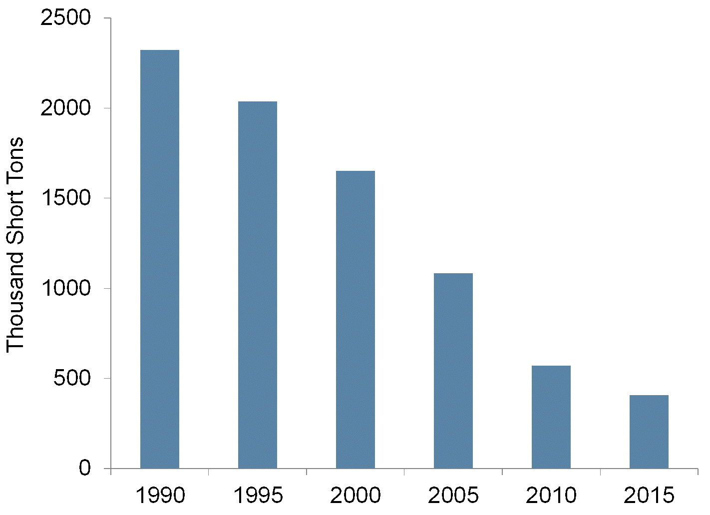
The emission reductions achieved under these programs have resulted in a substantive improvement in air quality as demonstrated by air pollutant concentrations measured by CASTNET and other cooperating networks. By 2015, EGUs required to comply with the ARP and/or CSAPR had reduced their SO2 emissions to 2.2 million short tons and NOx emissions to about 1.4 million short tons, decreases of 86 and 79 percent, respectively, from 1990 levels.
Congress mandated in the 1990 CAAA that the U.S. Environmental Protection Agency (EPA) provide consistent, long-term measurements for determining relationships between changes in emissions and subsequent changes in air quality, atmospheric deposition, and ecological effects. CASTNET operated 95 monitoring stations in 2015 throughout the contiguous United States, Alaska, and Canada. EPA and the National Park Service (NPS) are the primary sponsors of CASTNET. NPS began its participation in 1994 and operated 25 sites during 2015. The Bureau of Land Management-Wyoming State Office (BLM) operated five sites in Wyoming.
In 2015, a small footprint site was added to tribal lands for the Nez Perce Tribe in Idaho (NPT006). A small footprint seasonal site was also established at the summit of Whiteface Mountain, NY (WFM007) to operate simultaneously with a cloud water collector operated by the New York State Department of Environmental Conservation (NYSDEC). WFM007 also operated during the summer of 2016 and will operate during the summer of 2017.
This report summarizes CASTNET monitoring and the resulting concentration and deposition data collected over the 26-year period from 1990 through 2015. Additional information, previous annual reports, other CASTNET documents, and the CASTNET database can be found on the EPA CASTNET website, https://www.epa.gov/castnet/. The website provides a complete archive of concentration and deposition data for all CASTNET sites.
Locations of Monitoring Sites
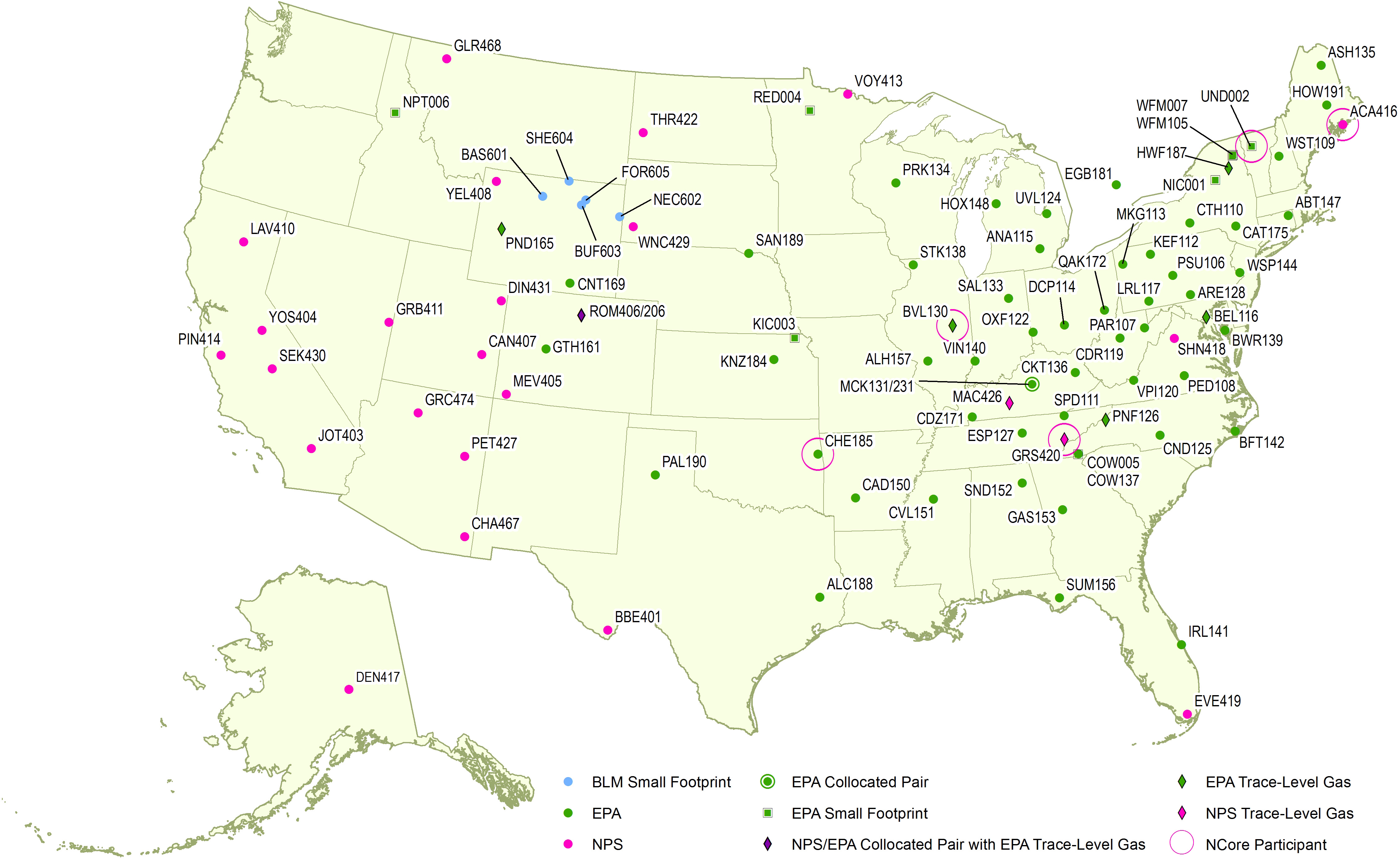
The locations of the CASTNET monitoring sites that were operational during 2015 are depicted in Figure 1-1. Ninety-five monitoring sites were operated at 93 distinct locations. To estimate precision across the network, co-located sites were operated at Mackville, KY (MCK131/231) and Rocky Mountain National Park, CO (ROM406/206) during 2015. The ROM406/206 pair ensures consistency between EPA (ROM206) and NPS (ROM406). Of the two Rocky Mountain monitoring sites, ROM406 is specified as the regulatory monitoring site for O3. Appendix A provides the location of each site and includes information on start date, latitude, longitude, elevation, identification of the nearby National Atmospheric Deposition Program (NADP) site, land use, terrain type, operating agency, and if the site is a reference site used for trends. Two new sites (NPT006, ID and WFM007, NY) were added to the network during 2015.
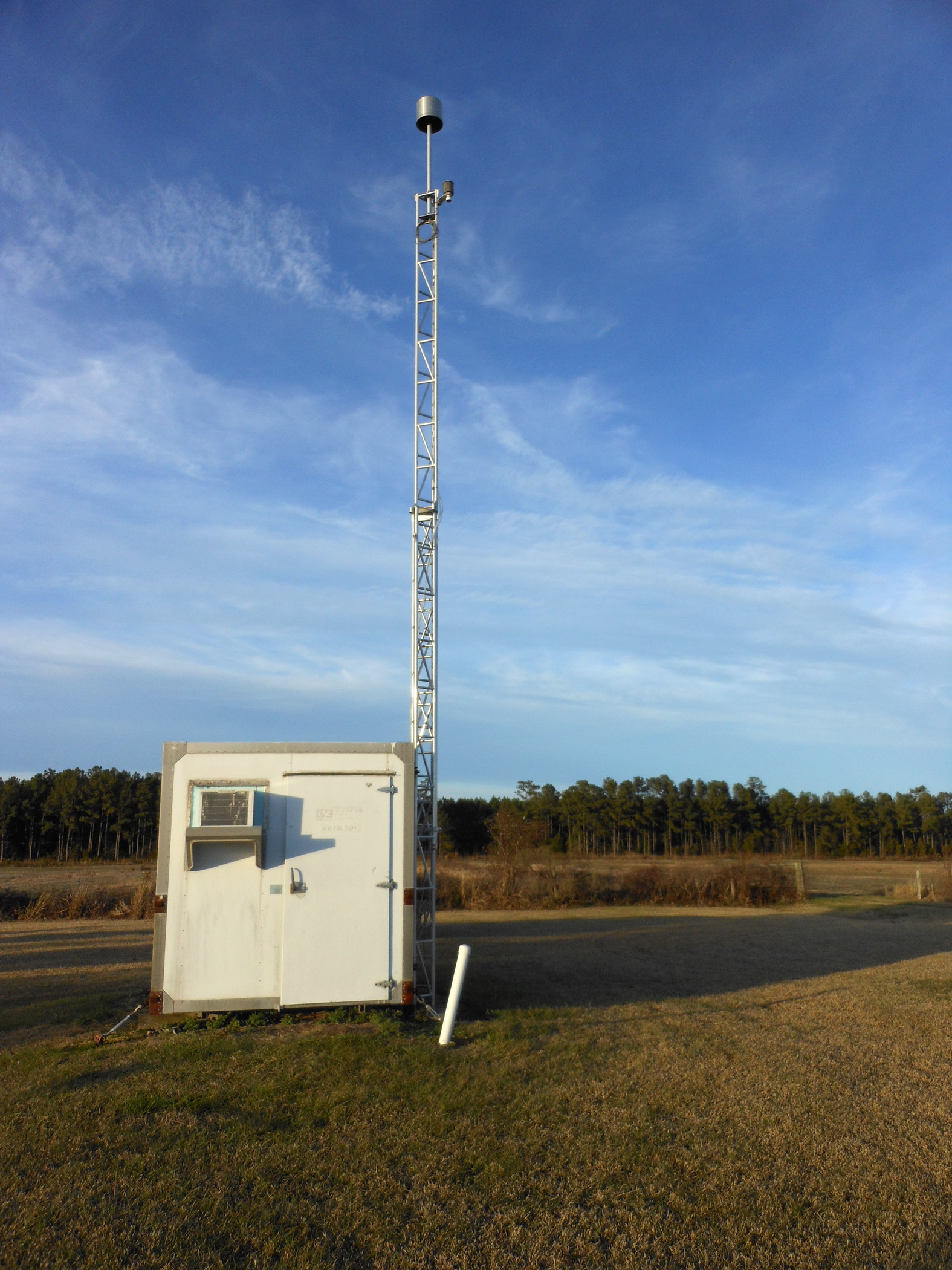
Beaufort, NC (BFT142)
Measurements Recorded at CASTNET Sites
All CASTNET sites measure weekly ambient concentrations of acidic pollutants, base cations, and chloride (Cl -) using a 3-stage filter pack with a controlled flow rate (Amec Foster Wheeler, 2014). Gaseous pollutant concentrations include SO2 and nitric acid (HNO3). Particulate concentrations include sulfate (SO42-), nitrate (NO3-), ammonium (NH +), magnesium (Mg 2+), calcium (Ca 2+), potassium 434 (K +), sodium (Na +), and Cl -. The filter pack is exchanged each Tuesday and shipped to the analytical chemistry laboratory for analysis. Ambient temperature is measured at 9 meters (m) at all sites in part to enable conversion of concentrations to local conditions.
Most CASTNET sites include a temperature-controlled shelter and continuous O3 monitoring system. The O3 inlet and filter pack are located atop a 10-m tower. Some CASTNET sites also measure trace- level SO2, carbon monoxide (CO), and nitrogen oxide/total reactive oxides of nitrogen (NO/NOy). In 2015, meteorological parameters were measured at 6 EPA-, 25 NPS-, and 5 BLM-sponsored CASTNET sites. Measured meteorological parameters include 2-m temperature, wind speed and direction, standard deviation of the wind direction, solar radiation, relative humidity, precipitation, and surface wetness (at select sites).
Cooperating Networks
CASTNET monitors air quality and deposition in cooperation with other national and international networks. EPA uses CASTNET and these other long-term national networks to assess the effectiveness of emission control programs.
NADP operates:
- National Trends Network (NTN), which includes about 269 monitoring stations with wet deposition samplers to measure the concentrations and deposition rates of air pollutants removed from the atmosphere by precipitation. NTN operates wet deposition samplers at or near virtually every CASTNET site.
- Ammonia Monitoring Network (AMoN), which operates passive ammonia (NH3) samplers at 103 sites with 68 of the AMoN sites at or near CASTNET locations. AMoN, in operation since 2007, provides information on 2-week integrated NH3 concentrations.
- Mercury Deposition Network (MDN), which operates 113 samplers to measure mercury (Hg) in precipitation. MDN samplers are operated at several CASTNET sites.
- Atmospheric Mercury Network (AMNet), which measures atmospheric concentrations of gaseous oxidized, particulate-bound, and elemental Hg at 24 locations in the continental United States, Canada, Hawaii, and Taiwan in order to estimate dry and total Hg deposition.
NADP’s website gives detailed information on each of these sub-networks: http://nadp.isws.illinois.edu/.
Canadian Air and Precipitation Monitoring Network (CAPMoN) operates 33 measurement sites throughout Canada and one in the United States. CASTNET and CAPMoN both operate filter pack samplers in Egbert, Ontario, Canada. CAPMoN operates a wet deposition sampler at the Pennsylvania State University CASTNET site (PSU106, PA).
EPA’s National Core Monitoring (NCore) reports on particulate matter (PM) mass; PM species; O3, SO2, NO/NOy, and CO concentrations; and meteorological parameters at approximately 80 sites. Five rural NCore sites are co-located with CASTNET sites.
BLM’s Wyoming Air Resources Monitoring System (WARMS) operates eight sites and the meteorological system at one of the CASTNET sites, Pinedale (PND165), in Wyoming. Five of the WARMS sites are CASTNET-protocol sites (http://www.blmwarms.net/) and include meteorological measurements. Two sites include O3 monitoring.
Interagency Monitoring of Protected Visual Environments (IMPROVE) measures speciated aerosol pollutants that affect visibility near more than 20 CASTNET sites. For more information on IMPROVE, see http://vista.cira.colostate.edu/IMPROVE/.
Quality Assurance Program
The CASTNET Quality Assurance (QA) program was established to ensure that all reported data are of known and documented quality in order to meet CASTNET objectives. The QA program also ensures intra-network consistency and comparability and the delivery of data that are reproducible and comparable with data from other monitoring networks. The 2015 QA program elements are documented in the CASTNET Quality Assurance Project Plan (QAPP; Amec Foster Wheeler, 2014). The QAPP includes standards and policies for all components of project operation, from site selection through final data reporting, with appendices that provide standard operating procedures for CASTNET operations.
Data quality indicators (DQI) such as precision, accuracy, and completeness are used to assess CASTNET measurements and supporting activities. Routine assessment and analysis help guarantee the production of high-quality data and information to meet project objectives. Measurements taken during 2015 and historical data collected over the period 1990 through 2014 were analyzed relative to DQI and their associated metrics. Results from these analyses are available in quarterly and annual QA reports posted on the EPA CASTNET website: https://www.epa.gov/castnet/. Selected analyses are summarized in callout boxes labeled, “QA Program Summary,” throughout this report.
Estimating Dry, Wet, and Total Deposition
Total deposition was assessed using the NADP’s Total Deposition Hybrid Method (TDEP; EPA, 2015c; Schwede and Lear, 2014), which combines data from established ambient monitoring networks and chemical-transport models. To estimate dry deposition, ambient measurement data from CASTNET and other networks were merged with dry deposition rates and flux output from the Community Multiscale Air Quality (CMAQ) modeling system. Wet deposition estimates were derived from precipitation chemistry measurements and precipitation amounts from the Parameter-elevation Regressions on Independent Slopes Model (PRISM). Dry and wet deposition fluxes were added to obtain the estimates of total deposition that are discussed in Chapters 9 and 11.
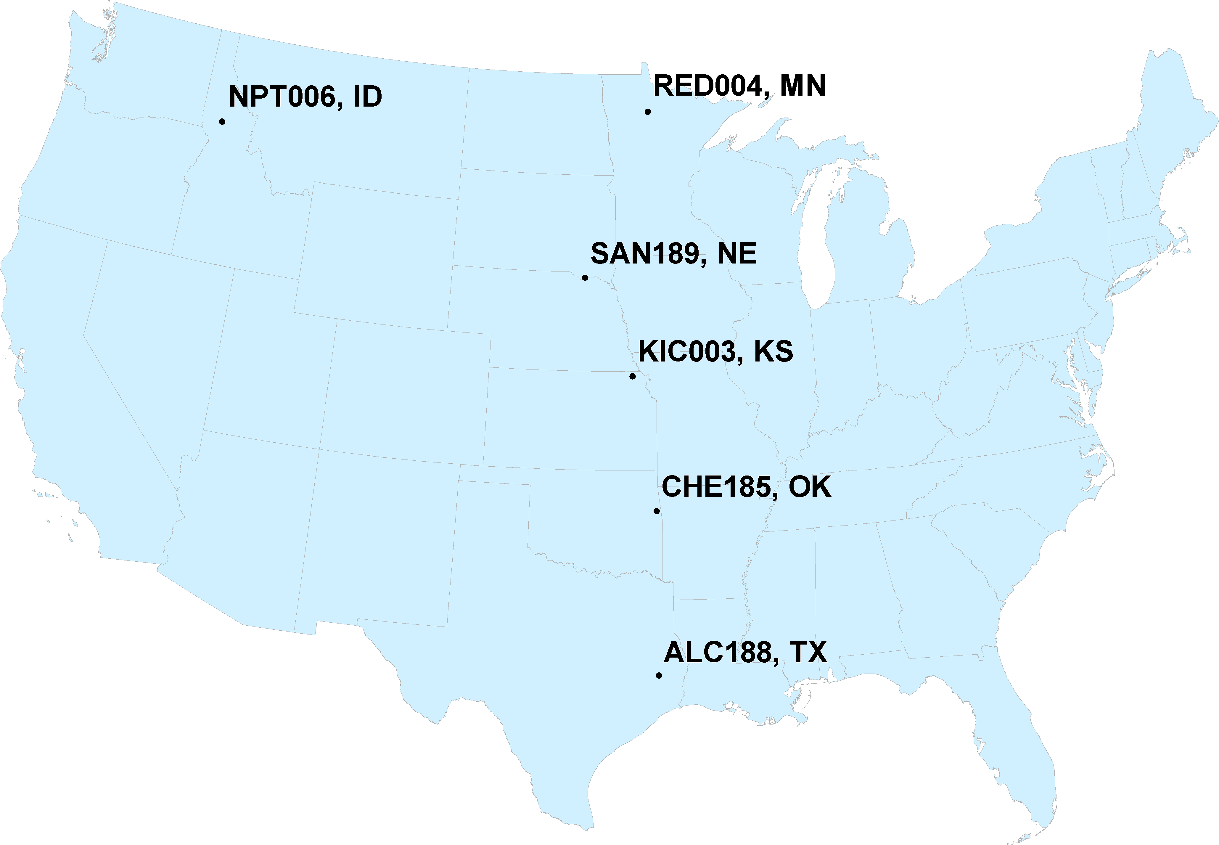
Building Tribal Partnerships with CASTNET Monitoring Sites
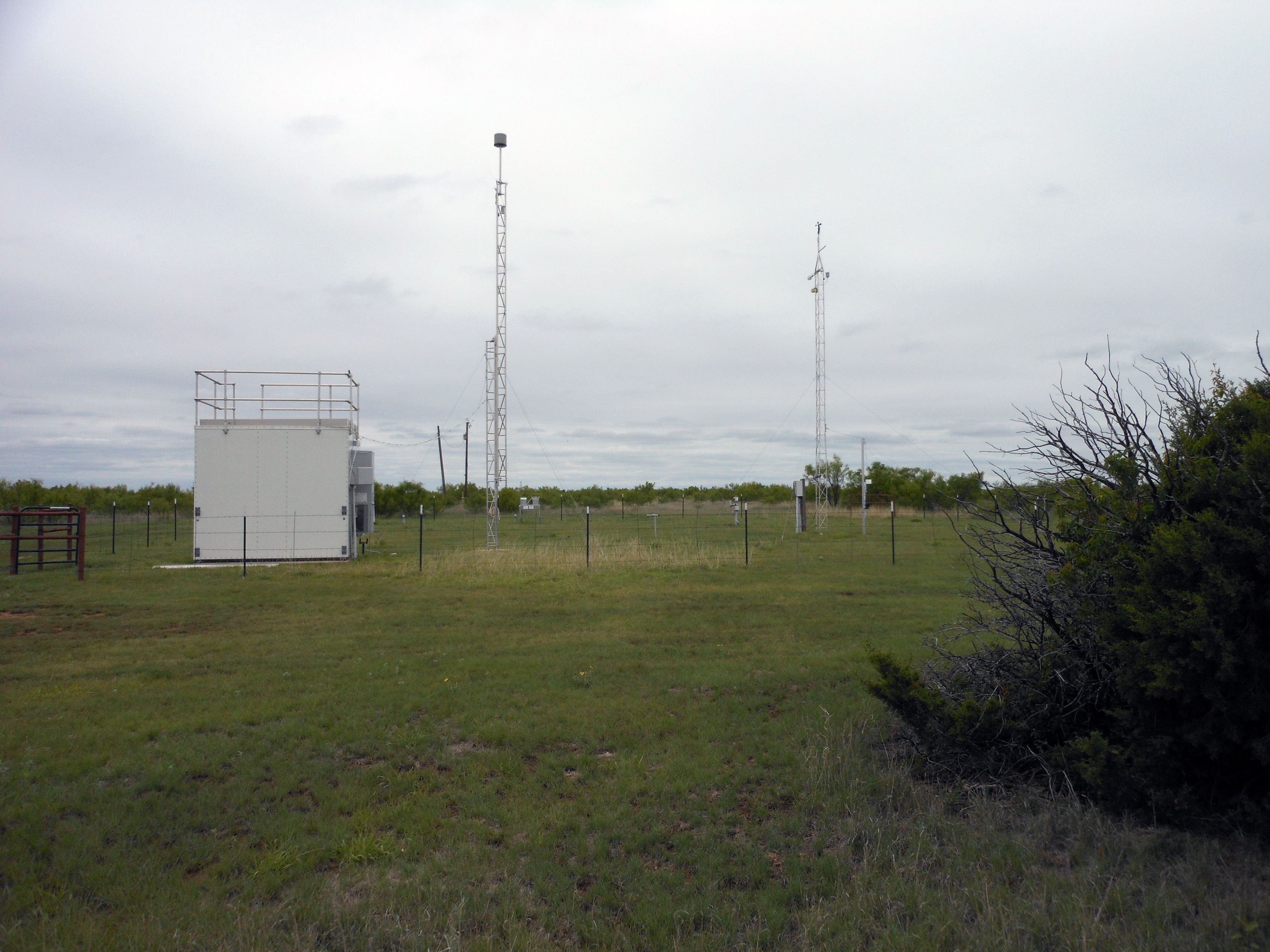
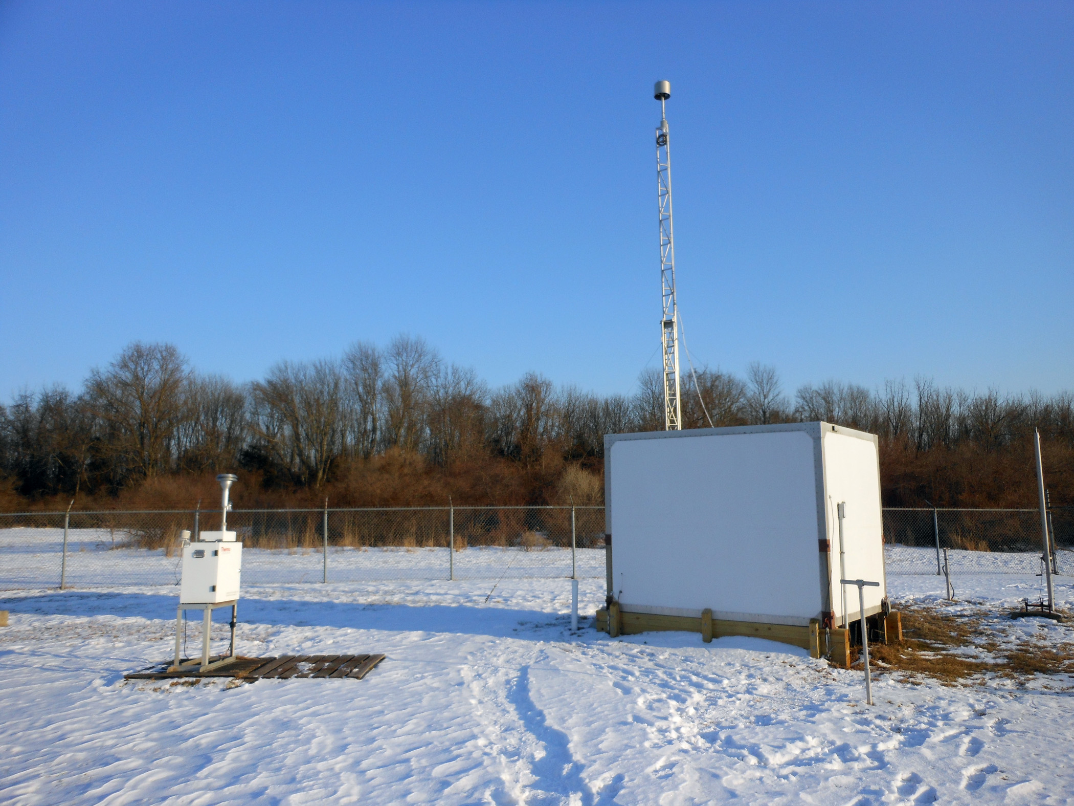
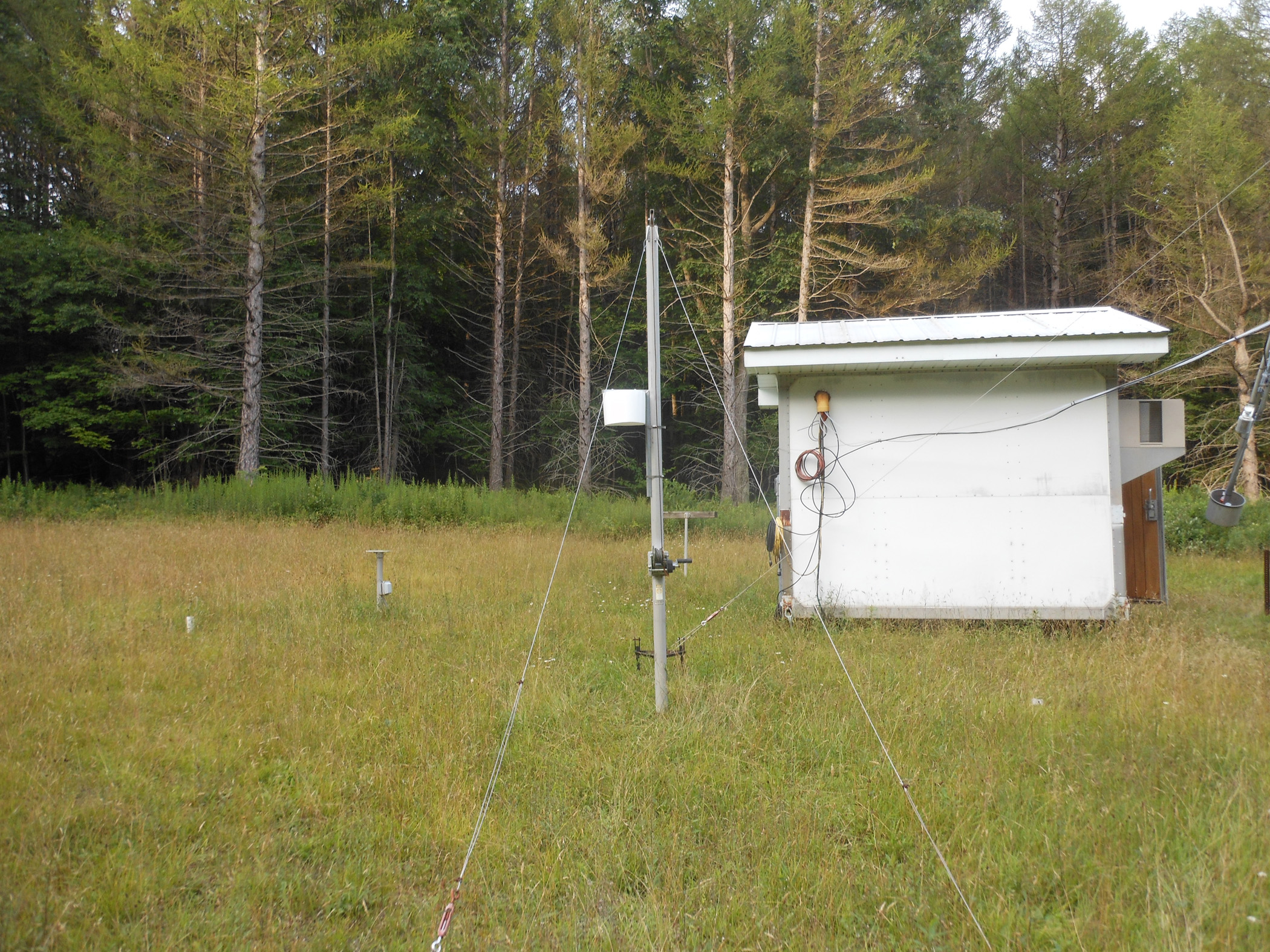
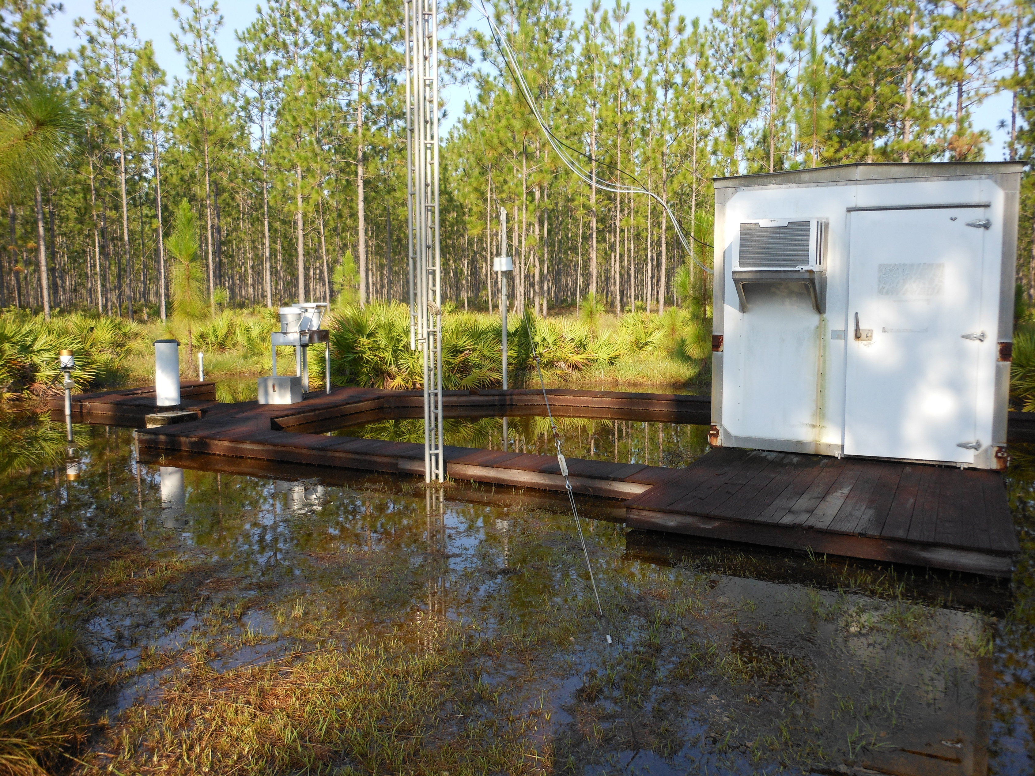
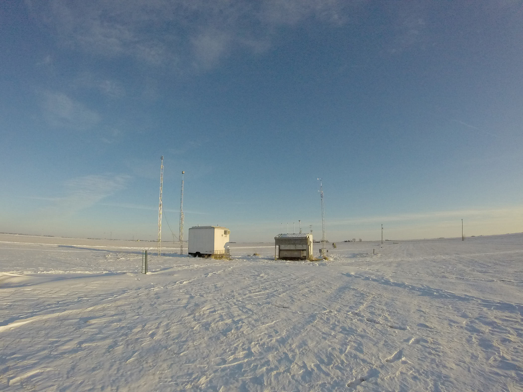
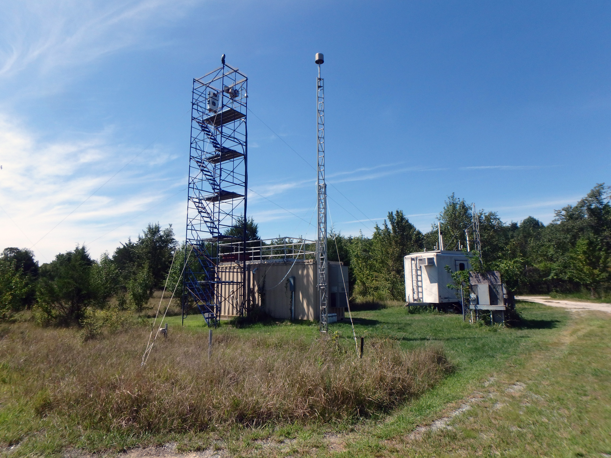
EPA partners with Cherokee Nation in Oklahoma, the Alabama-Coushatta Tribe in Texas, the Santee Sioux Tribe in Nebraska, Kickapoo Tribe in Kansas, the Red Lake Band of Chippewa Indians in Minnesota, and the Nez Perce Tribe in Idaho to operate CASTNET sites on tribal lands. In 2012, CASTNET developed a small footprint monitoring station that does not require a temperature-controlled shelter. The new type of monitoring station includes a 10-m sampling tower, filter pack sampling system, and data acquisition system (Figure 1-2), which can be operated off the grid. The new site design has produced cost savings and increased efficiency in terms of installation and power. The advent of the small footprint monitoring station has opened opportunities for new partners, such as the Nez Perce Tribe in Idaho, to participate in the CASTNET monitoring program. EPA may support additional tribal groups that are interested in establishing small footprint sites in order to assess sulfur and nitrogen inputs to their surrounding ecosystems.
Figure 1-2 Small Footprint Site Operated by Nez Perce Tribe in Idaho (NPT006)
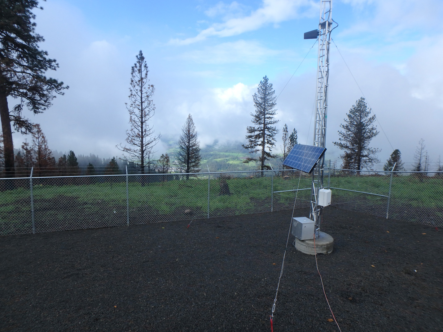
Tower with solar panel and equipment box
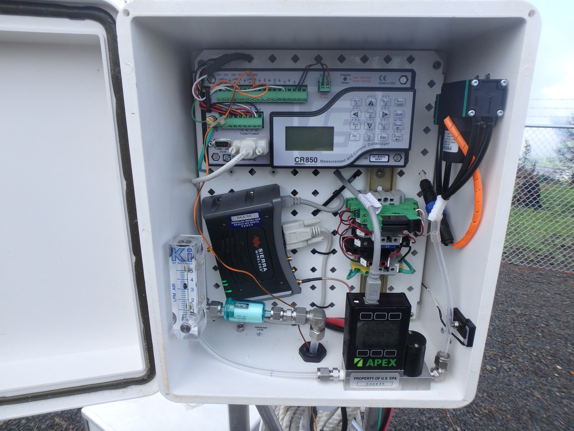
Interior of equipment box
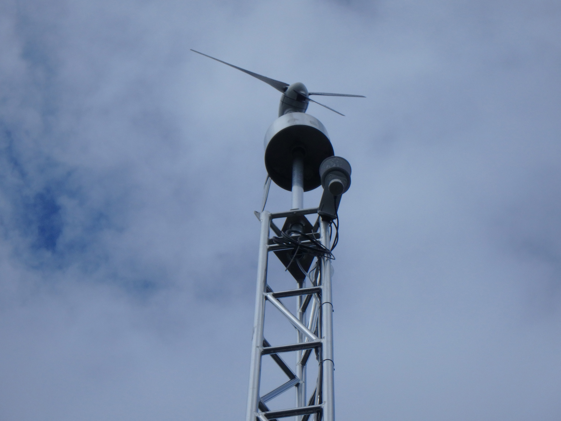
Filter pack sampling enclosure and wind turbine
The operation of CASTNET monitoring sites on tribal lands provides benefits to both the tribes and EPA. CASTNET measurements provide data on atmospheric pollutants and pollutant deposition to areas important to tribes. The measurements help the tribes understand the environmental effects of prescribed burns, wild fires, and nearby point or urban sources. When a CASTNET site is operated by a tribe, the equipment, training, QA, and data reporting are managed and funded by EPA, which provides the tribe with assurance that there will be no significant maintenance or repair costs and allows the tribe to begin or continue to build monitoring capacity.
For EPA, partnerships are important for operating a consistent, stable, long-term monitoring network. Current tribal sites fill in spatial gaps in the network within the central and northwest United States (Figure 1-3), and tribes provide much needed support for operations and infrastructure. Many tribal sites operate co-located monitoring instruments on behalf of NCore, NTN, MDN, AMNet, and AMoN. The Cherokee, Alabama-Coushatta, and Santee Sioux tribal sites provide regulatory O3 data to AIRNow and EPA’s Air Quality System (AQS).
Quality Assurance Program Results
Laboratory Intercomparison Results
During 2015, the Amec Foster Wheeler CASTNET laboratory participated in the Environment Canada (ECAN) Proficiency Testing (PT) Program for Inorganic Environmental Substances. The ECAN PT program conforms to the requirements of the American Association for Laboratory Accreditation (A2LA). The program meets the International Organization for Standardization (ISO)/International Electrotechnical Commission (IEC) 17043:2010 conformity assessment – general requirements for proficiency testing with scope of accreditation 2867.01. The Amec Foster Wheeler laboratory is one of 32 laboratories that participated in the 2015 Rain and Soft Waters round robin studies. The PT study samples consist of natural waters supplied by the National Laboratory for Environmental Testing. The CASTNET laboratory receives 10 samples of mixed rain and Canadian Shield waters for chemical analysis from ECAN every 6 months. The laboratory reported the eight CASTNET parameters for samples in two studies (study codes 0106 and 0107) during 2015.
The results reported by the 32 laboratories are evaluated for systematic bias and precision. Systematic bias is assessed using the Youden (1969) non-parametric analysis, while precision is calculated using algorithm A from the ISO standard 13528 (ISO, 2005).
Individual sample results are flagged based on the robust standard deviation obtained from the ISO 13528 computation (ISO, 2005). Samples within two standard deviations of the assigned (median laboratory) value are not flagged; samples between two and three standard deviations are given a warning flag; and samples greater than three standard deviations from the assigned value are flagged as above the action limit (remedial action is required). Laboratory results are considered systematically biased when individual parameters are ranked by the Youden analysis to be consistently and significantly higher or lower than the assigned value without regard to flagged results.
The CASTNET laboratory’s 2015 ECAN results for the eight CASTNET parameters are presented in Table 1-a. The overall laboratory performance rating was “Very Good” for both studies.
Cherokee Nation (Stilwell), OK (CHE185)
Table 1-a Amec Foster Wheeler Results for Studies 0106 and 0107
| Test Parameter | Analytical Method | Reference Method | Laboratory Performance Rating* | |
|---|---|---|---|---|
| Very Good: Study 0106 Summer 2015 | Very Good: Study 0107 Winter 2015 | |||
| Ammonia | AC | EPA Method 350.1 | Bias could not be assessed† | -0.8 percent | 0.0085 |
| Calcium | ICP-OES | EPA Method 6010 | Ideal | Ideal |
| Chloride | IC | EPA Method 300.0 | 0.7 percent | 0.0180 | Ideal |
| Magnesium | ICP-OES | EPA Method 6010 | Ideal | Ideal |
| Nitrate + Nitrite | IC | EPA Method 300.0 | Ideal | Ideal |
| Potassium | ICP-OES | EPA Method 6010 | Ideal | Ideal |
| Sodium | ICP-OES | EPA Method 6010 | Ideal | Ideal |
| Sulfate | IC | EPA Method 300.0 | Ideal | 1.6 percent | 0.0214 |
Note: *Expressed as bias percent slope (percent deviation of test results from assigned values) | y-intercept. Ideal slope = 1 | y- intercept = 0. Any result not 1 | 0 is reported as biased by ECAN. The CASTNET laboratory is accredited by A2LA to ISO/IEC 17025:2005 for a scope that includes the study parameters for methods used by the laboratory. The laboratory’s proficiency testing plan requires action for individual test results that are greater than three standard deviations from the assigned value, bias 5 percent or higher for a single parameter, three or more biased results of any magnitude in a single study, or a consecutive study result indicating bias of any magnitude for a given parameter.
†Seven of the 10 assigned values were below the laboratory limit of quantitation.
AC=automated colorimetry
ICP-OES=inductively coupled plasma-optical emission spectrometry
IC=ion chromatography
Source: Environment Canada (2015; 2016)
The overall laboratory rating indicates a percent score as described in Table 1-b. The five-year historical laboratory rating is listed by ECAN as “Very Good.”
Table 1-b Laboratory Performance Rating from 2011–2015
| Laboratory Performance Rating | |
|---|---|
| Rating | Percent Score* |
| Very Good | 0 - 5 |
| Good | > 5 - 12.5 |
| Fair | > 12.5 - 30 |
| Poor | > 30 |
*Sum of parameters biased and results flagged
Source: Environment Canada (2015; 2016)
Chapter 2: Ozone Concentrations
CASTNET is the principal network for monitoring rural, ground-level ozone concentrations in the United States and producing critical information on geographic patterns in rural ozone levels. Ozone data measured at 80 CASTNET sites from 2013 through 2015 were evaluated with respect to the National Ambient Air Quality Standards (EPA, 2008) and used to calculate design values, which are defined in Title 40 Code of Federal Regulations Part 50 Appendix U (EPA, 2015a). Maps of 3-year averages of fourth highest daily maximum 8-hour average (DM8A) ozone concentrations for 2013 through 2015 and fourth highest DM8A ozone concentrations for 2015 are presented. Trends in fourth highest DM8A ozone concentrations for eastern and western reference sites are shown using box plots.
In 2015, hourly average concentrations were measured at 80 CASTNET sites. These data are archived in the CASTNET database and delivered routinely to the EPA AQS. Data from these sites, with the exception of Howland, ME (HOW191) and the co-located sites at MCK231, KY and ROM206, CO, which are designated as non-regulatory, are used to calculate fourth highest DM8A concentrations when three years of Title 40 Code of Federal Regulations (CFR) Part 58-compliant data become available. CASTNET measurements provide information that is essential for evaluating rural O3 concentrations in the context of the O3 NAAQS and in terms of presenting information on trends and geographic patterns in regional O3.
A design value is a statistic that describes the air quality status of a given area relative to the concentration values required by the NAAQS. Design values change as each new 3-year period of monitored ozone concentrations becomes available. Design values are used to classify nonattainment areas, assess progress towards meeting the NAAQS, and develop control strategies to achieve the NAAQS. For example, if 3-year averages of 2013–2015 fourth highest DM8A ozone concentrations are used for purposes of attainment designation and exceed 0.075 parts per million (ppm), then ozone concentrations will have to be reduced to 0.075 ppm or below to achieve the 2008 ozone NAAQS. Designated criteria pollutant nonattainment areas are provided on the EPA website.
The information presented in this chapter includes maps and trends in the annual fourth highest DM8A O3 concentrations measured at CASTNET sites. Additional maps of O3 concentrations from the NPS Air Atlas can be viewed at http://nature.nps.gov/air/maps/airatlas/index.cfm and http://nature.nps.gov/air/data/products/parks/index.cfm.
Measurements from 34 eastern and 16 western reference sites (see Appendix A) were analyzed to determine trends in O3 concentrations. These sites were also used to show trends in ambient nitrogen and sulfur concentrations (Chapters 4 and 6). The eastern reference sites have been reporting CASTNET measurements since at least 1990 and the western reference sites since at least 1996.
2008 National Ambient Air Quality Standards for Ozone
| Ozone 1 | Primary Standard | Secondary Standard | |
|---|---|---|---|
|
Level |
Averaging Time |
Level |
Averaging Time |
|
0.075 ppm 1 |
8-hour 2 |
0.075 ppm 1 |
8-hour 2 |
Note:
1 The NAAQS was revised from 0.075 ppm to 0.070 ppm on October 1, 2015.
2 To attain this standard, the 3-year average of the fourth highest DM8A O3 concentrations measured at each monitor within a specified area must not exceed 0.075 ppm or 75 parts per billion (ppb) in practice (effective May 27, 2008; EPA, 2008). O3 concentrations are commonly presented in units of ppb.
The primary O3 NAAQS is designed to protect public health. The secondary standard is designed to protect public welfare and the environment. Both O3 NAAQS are set at a level of 0.075 ppm averaged over eight hours for the annual fourth highest value.
For the primary and secondary standards, EPA uses the pollutant indicator (O3), forms (fourth highest daily maximum averaged across three consecutive years), and averaging time (eight hours; EPA, 2008). The secondary standard is equivalent, based on the W126 index, to a level of protection of 17 ppm-hour or lower averaged over three years (EPA, 2008). The W126 index is a weighted index designed to reflect the cumulative exposures that can damage plants and trees during the consecutive three months in the growing season when daytime O3 concentrations are the highest and plant growth and production are most affected (Lefohn and Runeckles, 1987).
The EPA and other federal, tribal, state, and local agencies measure O3 concentrations on an hourly basis through national and local monitoring programs. Amec Foster Wheeler followed EPA procedures (2015a) to estimate O3 design values and 2015 fourth highest DM8A O3 concentrations at CASTNET sites. Measurements potentially affected by exceptional events were not removed when calculating these estimates. “Exceptional events are unusual or naturally occurring events that can affect air quality but are not reasonably controllable using techniques that state, tribal, or local air agencies may implement in order to attain and maintain the NAAQS” (EPA, 2016). The Exceptional Events Rule was updated on October 3, 2016 1 (epa.gov/air-quality-analysis/exceptional-events-rule-and-guidance) and provides the requirements for excluding air quality data from regulatory decisions if the data are affected by events outside an agency’s control, such as a wildfire or stratospheric intrusion.
CASTNET O3 data are used to gauge compliance with the NAAQS at EPA-, NPS- and BLM- sponsored sites that were 40 CFR Part 58 compliant for the years 2013 through 2015.
Note: 1 A revised Exceptional Events Rule was posted for public comment on 9/16/2016.
Quality Assurance Program Results
Ozone Concentrations
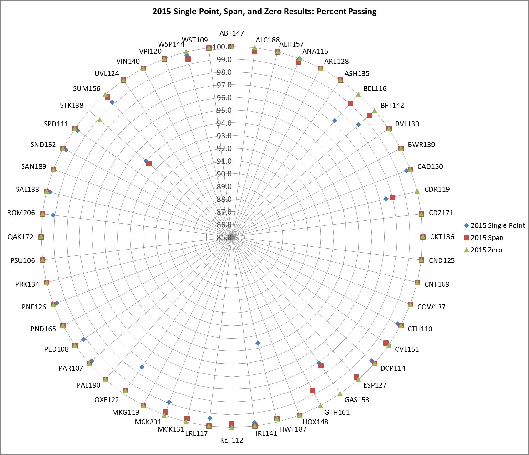
Ozone quality control (QC) criteria are set forth in 40 CFR Part 58, Appendix A (EPA, 2013). Figure 2-a presents summary statistics of critical criteria measurements at O3 sites for measurements collected during 2015. All data associated with QC checks that failed to meet the established criteria were invalidated unless the cause of failure was documented to have no effect on ambient data collection. QC failures for EPA- sponsored sites are addressed in quarterly QA reports, which can be found on the EPA CASTNET website.
Note:
QA program results for NPS-sponsored sites measuring O3 may be accessed here.
1 A revised Exceptional Events Rule was posted for public comment on 9/16/2016.

Prince Edward, VA (PED108)
Eight-Hour Ozone Concentrations
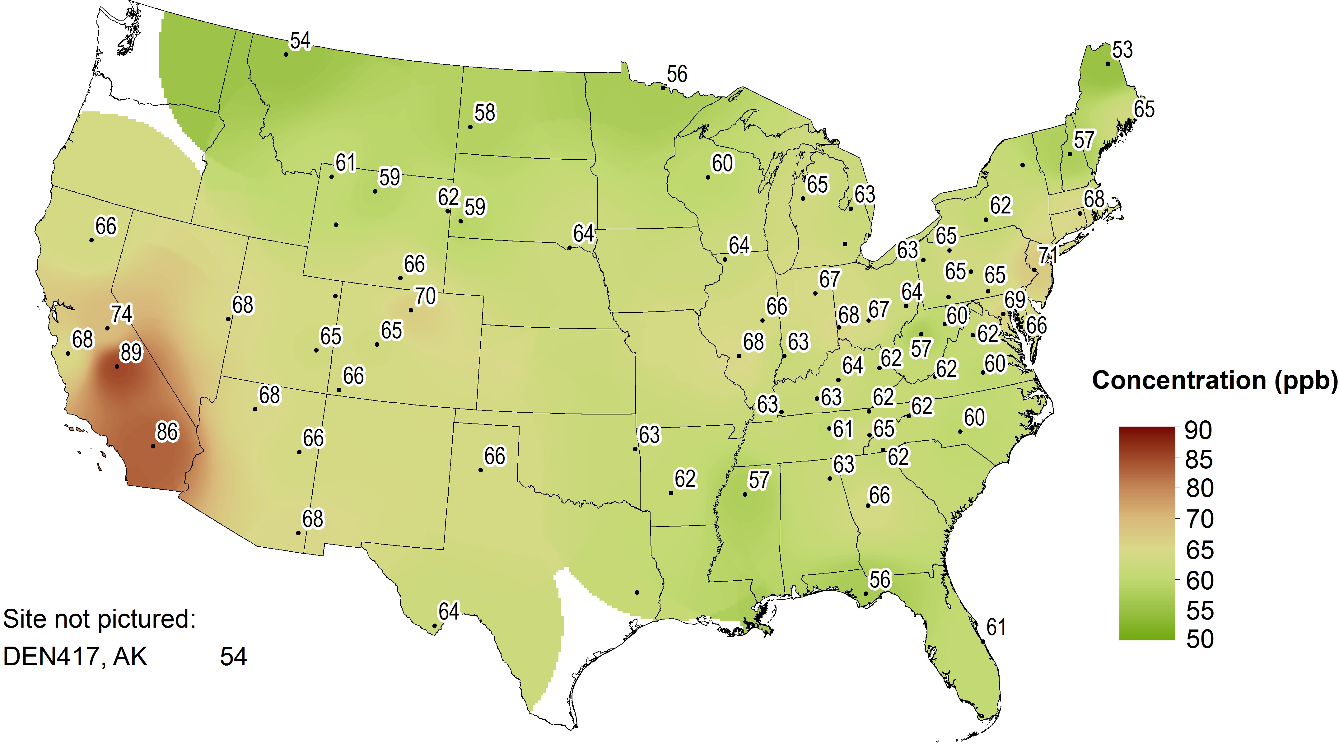
Regulatory-compliant procedures were used to measure all CASTNET O3 data for 2013 through 2015 and were used to calculate fourth highest DM8A O3 concentrations and to gauge compliance with the NAAQS, with the exception of sites HOW191, ME; MCK231, KY; and ROM206, CO. HOW191 does not meet regulatory siting criteria. MCK231 and ROM206 are co-located sites used solely for QA purposes and are designated as “NAAQS excluded.” O3 concentrations were not included on the maps in this chapter if the 3-year average was not available because of incomplete data; these sites are shown as dots with no value. Three-year averages of the fourth highest DM8A O3 concentrations for 2013 through 2015 are presented in Figure 2-1. Two California CASTNET sites measured fourth highest DM8A O3 concentrations above the 2008 NAAQS. The highest O3 concentration of 89 parts per billion (ppb) was sampled at the Sequoia and Kings Canyon National Parks, CA (SEK430) site. The highest eastern concentration (71 ppb) was measured at Washington Crossing, NJ (WSP144). Table 2-1 lists sites with 2013–2015 O3 design values greater than 75 ppb.
Figure 2-1 Three-year Average of Fourth Highest DM8A O3 Concentrations (ppb) for 2013–2015
 Download Image
Table 2-1 Sites with Design Values for 2013–2015 greater than 75 ppb
| Site ID | State | Sponsor | 30year Average |
|---|---|---|---|
| SEK430 | California | NPS | 89 |
| JOT403 | California | NPS | 86 |
All valid 2015 O3 concentrations that meet regulatory requirements are shown in Figure 2-2. During 2015, WSP144, NJ measured a fourth highest DM8A O3 concentration of 75 ppb. Two California sites measured fourth highest DM8A O3 concentrations greater than 75 ppb.
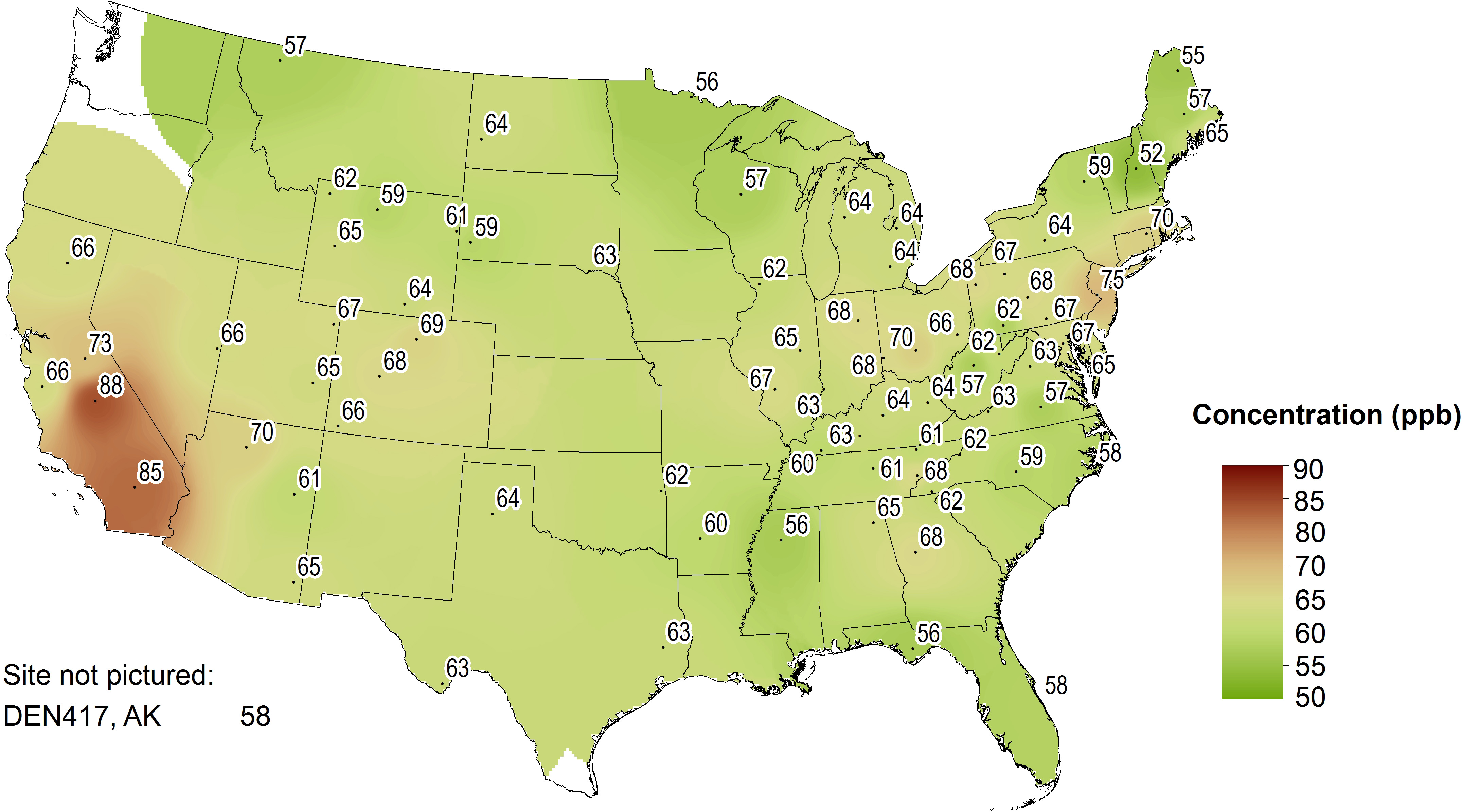
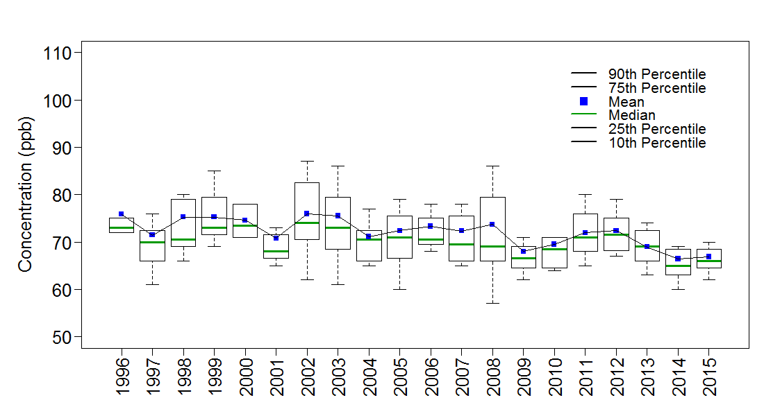
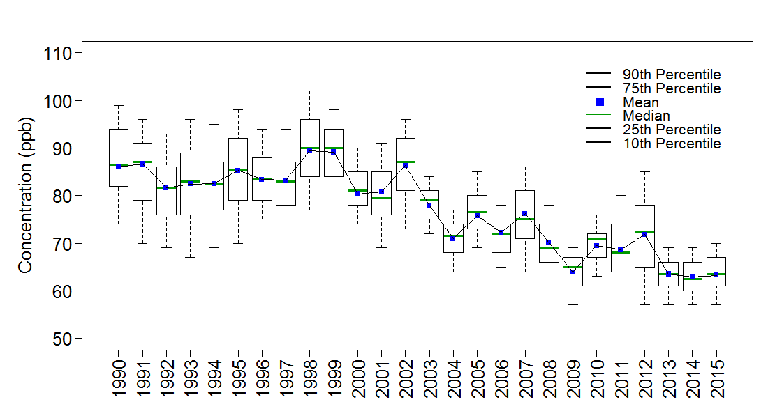
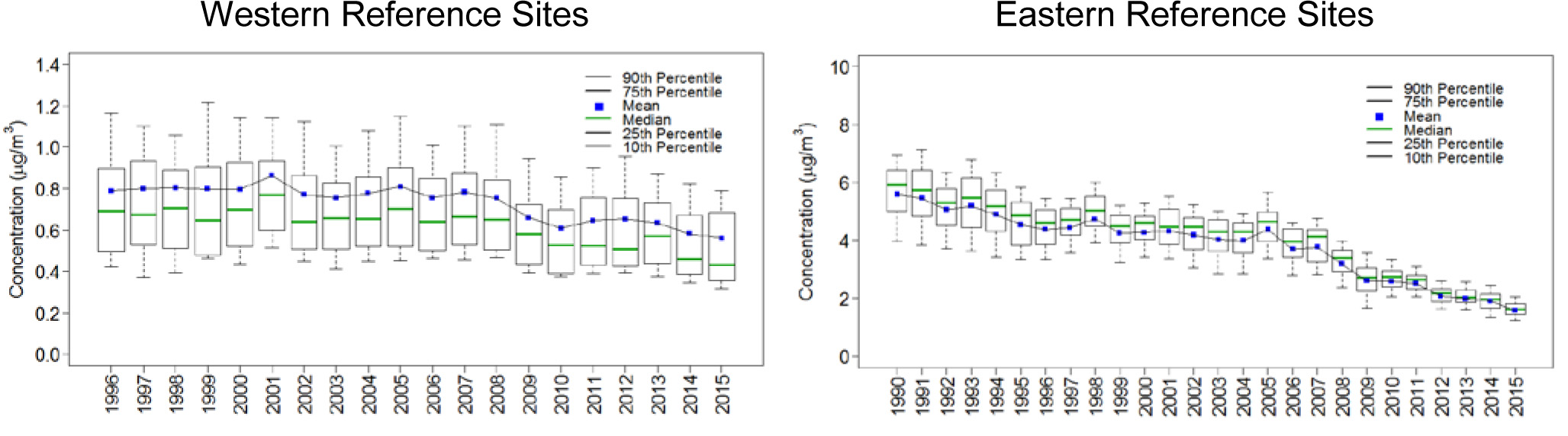
Figure 2-3 provides box plots depicting trends in 1-year mean, median, and annual distribution of fourth highest DM8A O3 concentrations from the eastern reference sites (right side) for 1990 through 2015 and for the western reference sites (left side) for 1996 through 2015. The reference sites were selected for their long-term data record and consistent performance. The eastern O3 data show an overall decline since 2002. There was an increase in fourth highest DM8A O3 concentrations from the 2009 minimum through 2012, followed by a decrease in 2013. The 2015 aggregate median data point, 63.5 ppb, is slightly higher than the 2014 value of 62.5 ppb, the lowest level in the history of the network.
The western O3 data also show an increase in fourth highest DM8A O3 concentrations from the 2009 minimum through 2012, followed by a decrease in 2013. The 2015 median of the fourth highest DM8A O3 concentrations for the western reference sites was 66 ppb.
Figure 2-3 Trends in Fourth Highest DM8A O3 Concentrations
Palo Duro Canyon State Park, TX (PAL190)
Chapter 3: Evaluating Elevated Ozone Concentrations Measured at Washington Crossing, New Jersey
CASTNET has operated a monitoring site at Washington Crossing, NJ (WSP144) since December 1988. The site frequently measures ozone concentrations that are higher than those measured at most CASTNET sites located in the eastern United States. Over the past two years, the annual fourth highest DM8A ozone concentrations exceeded 70 ppb. Elevated concentrations at this site were typically associated with regional episodes when high concentrations extend throughout the Mid-Atlantic and Northeast urban corridor.
CASTNET began operating a monitoring site at WSP144 in 1988 as part of the National Dry Deposition Network. The site (see Figure 1-1 for location and Appendix A for additional site details) is situated in Washington Crossing State Park approximately 1,000 feet northeast of the Delaware River. In addition to monitoring weekly pollutant concentrations, the O3 monitoring at the site helps the state of New Jersey meet the minimum required number of O3 monitoring sites within the Trenton-Ewing metropolitan statistical area, thereby fulfilling 40 CFR Part 58 Appendix D monitoring network design requirements. The monitoring site lies about 35 miles northeast of Philadelphia and 60 miles southwest of New York City—within the Mid-Atlantic and Northeast urban corridor. This broad region experiences some of the highest O3 concentrations in the eastern United States. While not as high as concentrations measured at some relatively nearby urban regulatory monitoring sites, which were designated nonattainment based on the 2008 O3 NAAQS, historical fourth highest DM8A O3 concentrations at WSP144 have exceeded the 2008 O3 NAAQS of 75 ppb (Table 3-1).
Table 3-1 Fourth Highest DM8A O3 Concentrations Measured at WSP144
| Year | Concentration (ppb) |
|---|---|
| 2015 | 75 |
| 2014 | 71 |
| 2013 | 69 |
| 2012 | 83 |
| 2011 | 80 |
| 2010 | 82 |
EPA works with state and tribal partners to understand air quality dynamics (i.e., the complex relationship between air quality, emissions, and weather) in order to reduce O3 concentrations in areas that exceed the O3 NAAQS 1. While not the focus of gauging the specific effects of emission reduction programs, such as CSAPR 2, CASTNET sites are well positioned for evaluating regional impacts of changes in O3 concentrations. Comprehensive Air Quality Model with Extensions (CAMx) modeling 3 indicated that, across all of the CASTNET sites, WSP144 received the highest percentage of contributions from upwind states totaling 65 percent of its projected 2017 O3 design value. New Jersey in-state emissions also affected this site.
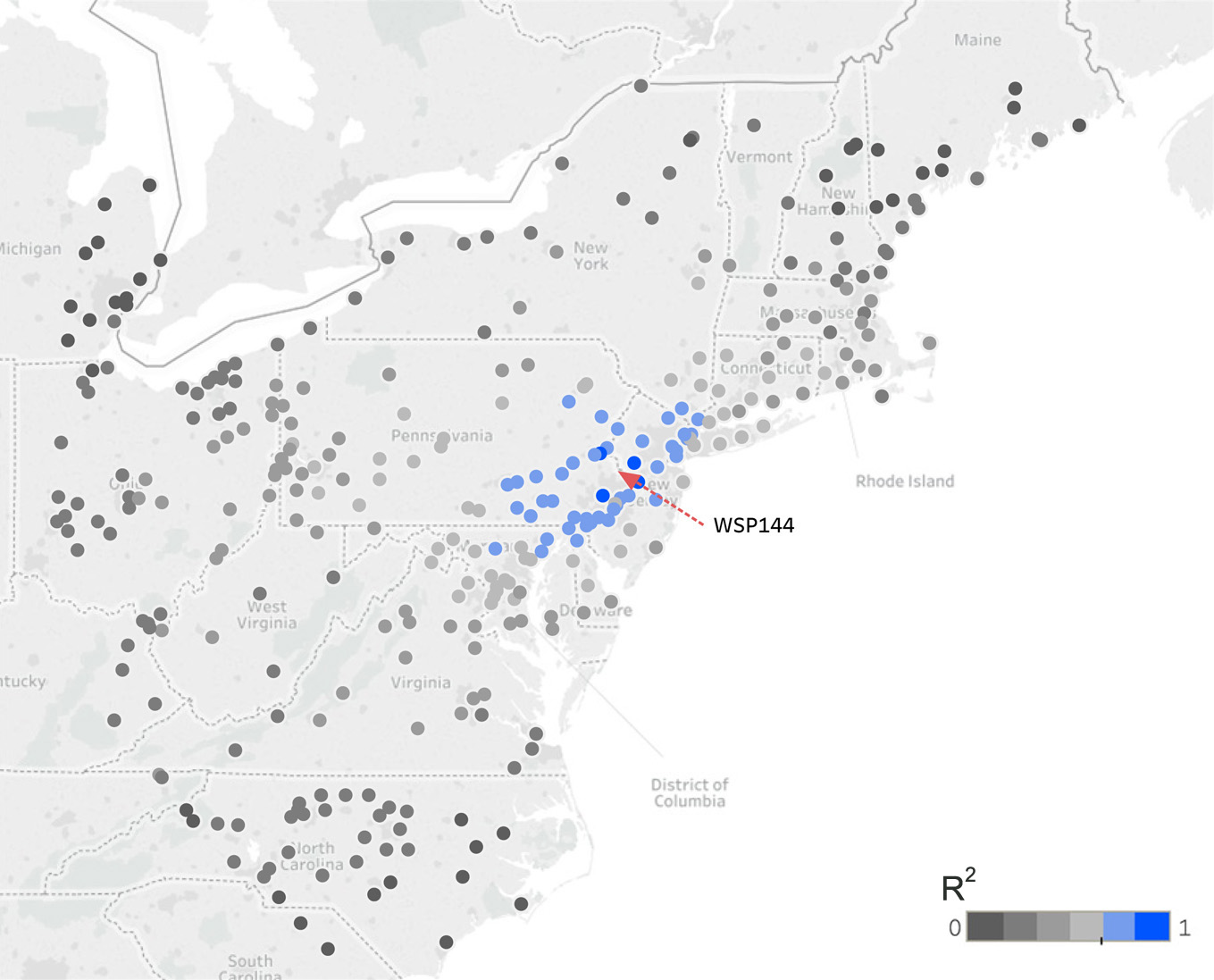
As with most CASTNET sites, WSP144 was sited to be representative of a region and minimally impacted by local sources. Washington Crossing’s immediate environs are characterized by a mix of parks, woods, and agriculture. Comparisons of O3 measurements collected at the WSP144 monitor with data from other regulatory O3 monitors within the Mid-Atlantic region suggest that the site does provide regionally representative measurements. Figure 3-1 displays coefficient of determination (R 2) values from a least squares linear regression comparison of the WSP144 DM8A values with DM8A values from surrounding regulatory O3 monitors within 800 kilometers (km) for the May 1 through October 31, 2015 O3 season. The color scale highlights the spatial extent where R 2 is highest (at or above 0.70) indicating that these sites often experience similar patterns of O3 concentrations. This area of strongest correlation spans the Eastern Seaboard from Maryland to Long Island, including central and western New Jersey. The strong correlation over this region is likely a result of similar emission and weather patterns. Nearby sites that exhibit a substantially weaker correlation suggest they are impacted by different emissions and weather conditions.
Washington Crossing (State Park), NJ (WSP144)
Figure 3-1 Regional Site-Level DM8A Comparisons with WSP144 (May 1–October 31, 2015)
 Download Figure
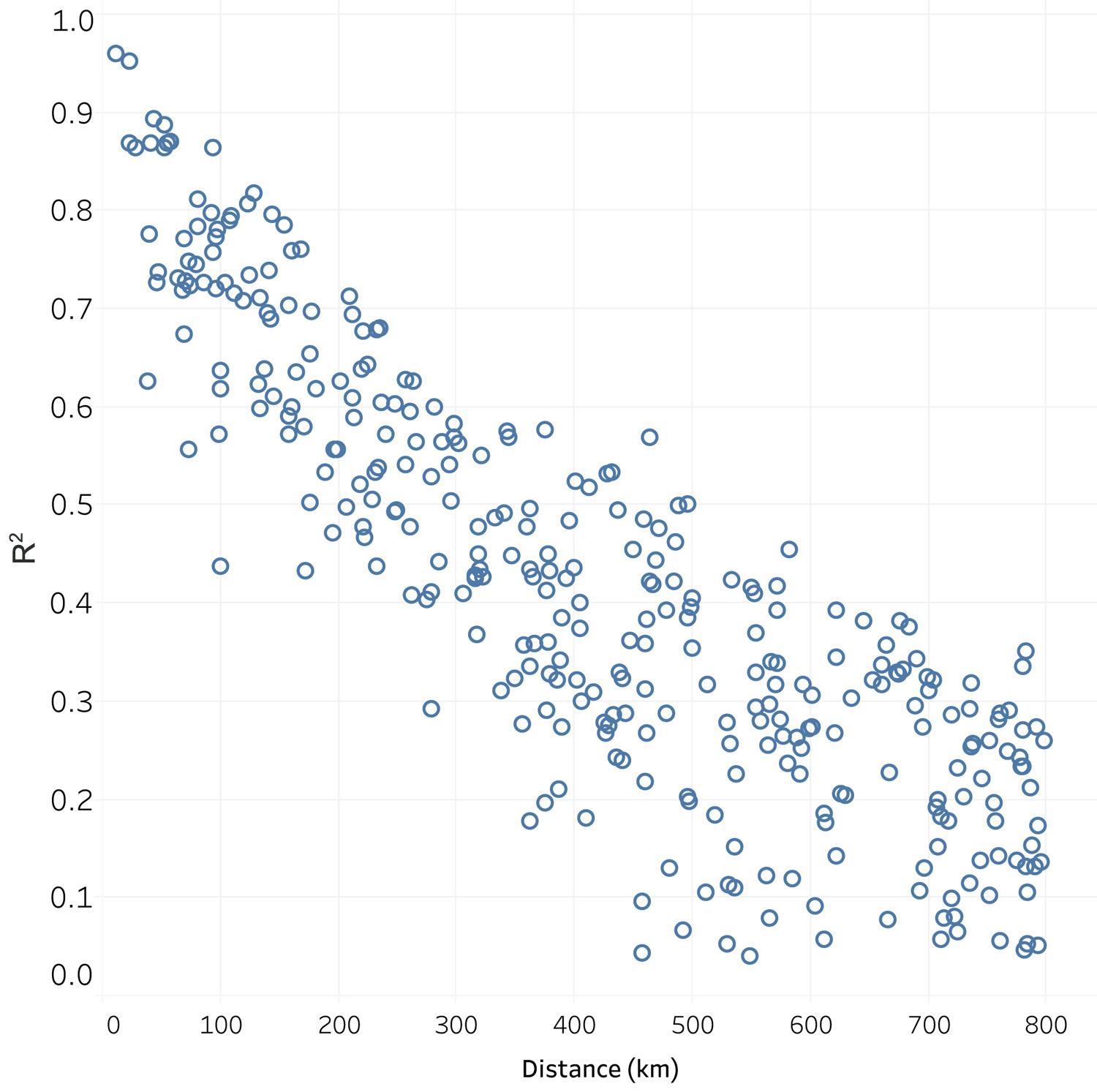
A comparison of the coefficients of determination between WSP144 DM8A values and DM8A values from other O3 monitors within the region is shown in Figure 3-2. The coefficient of determination for each monitor was calculated as a function of distance from WSP144. Typically, a monitor within 140 km of WSP144 had a coefficient of determination greater than or equal to 0.70. 4 A high coefficient was also calculated for a monitor located in Carroll County, Maryland (AQS number 24-013-0001), which is 209 km southwest of WSP144. Alternatively, some nearby sites did not meet the 0.70 criterion. For example, a site located in Philadelphia, PA (AQS number 42-101-0004), which is 39 km southwest of WSP144, had a DM8A R2 of 0.63 indicating that the Philadelphia monitor may be affected by both regional and local O3 pollution.
Figure 3-2 Regional Site-Level DM8A Comparisons with WSP144 by Distance (May 1–October 31, 2015)
 Download Figure
While Figure 3-2 displays correlation values for each monitoring site, DM8A data on individual days have to be analyzed to in order to understand the variable nature of weather patterns and the correlation with proximal monitors. The correlation patterns were different on an episode-by-episode basis. In any particular high DM8A episode, the correlation patterns varied depending on meteorological events. The eight days when DM8A levels exceeded 70 ppb during the 2015 O3 season are listed in Table 3-2. Elevated temperatures are known to play an important role (Camalier et al., 2007) in O3 formation. Therefore, maximum 1-hour temperature values and their percentiles are listed to help evaluate any effects temperature may have had on O3 on these days. The temperature measurements and statistics illustrate that four out of eight high DM8A episodes occurred when the maximum 1-hour temperature was within the 95th percentile for the 2015 O3 season. These results support the claim that elevated temperature is an important factor during these episodes, but they do not explain elevated O3 on moderate temperature days (e.g., May 8) or explain why other days with high temperatures (i.e., within the 95th percentile) did not have DM8A values above 70 ppb. Regional DM8A values measured at regulatory monitors on these eight days were then analyzed to better understand elevated O3 patterns.
Table 3-2 DM8A Levels Exceeding 70 ppb at WSP144 with Temperature and HYSPLIT 24-Hour Back Trajectory Distances
| Date | 2015 DM8A Concentration (ppb) | 2015 DM8A Concentration Rank | Maximum 1-Hour Temperature (Celsius) | Maximum 1-Hour Temperature Percentile | Average HYSPLIT Straight Line Distance (km) | Average HYSPLIT Curved Path Distance (km) |
|---|---|---|---|---|---|---|
| 05/08/2015 | 81 | 1 | 28.4 | 71 | 168 | 185 |
| 7/29/2015 | 81 | 1 | 32.6 | 99 | 146 | 174 |
| 6/11/2015 | 79 | 3 | 32.2 | 96 | 340 | 361 |
| 9/17/2015 | 75 | 4 | 29.1 | 77 | 116 | 145 |
| 9/18/2015 | 75 | 4 | 28.6 | 72 | 143 | 156 |
| 09/08/2015 | 74 | 6 | 33.1 | 99 | 244 | 307 |
| 09/02/2015 | 72 | 7 | 31.8 | 94 | 63 | 111 |
| 6/12/2015 | 71 | 8 | 32.2 | 96 | 193 | 261 |
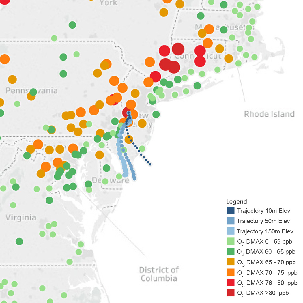
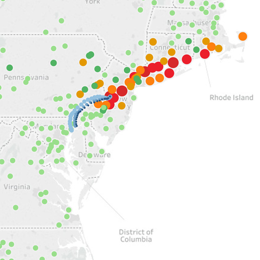
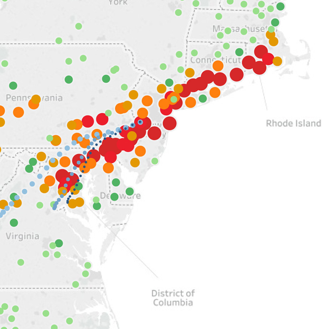
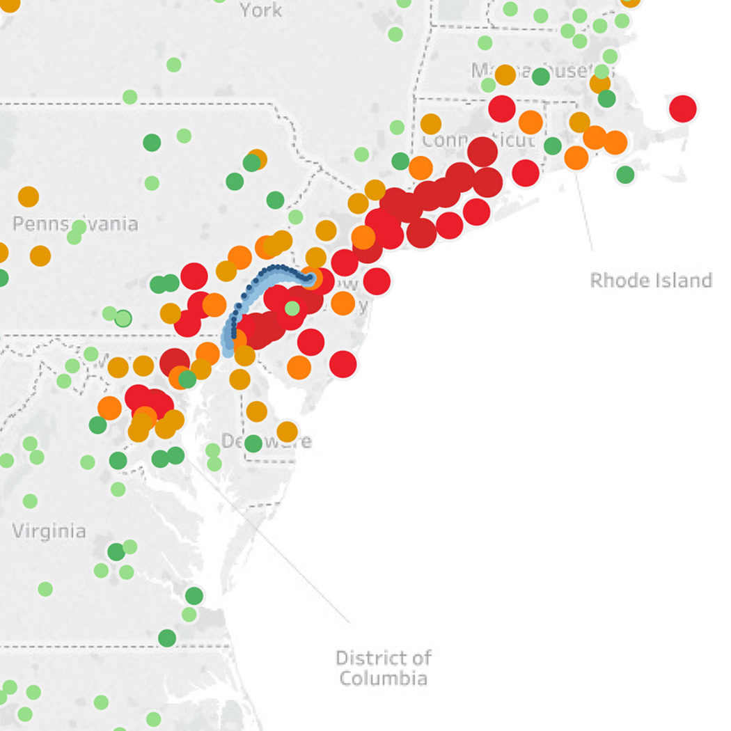
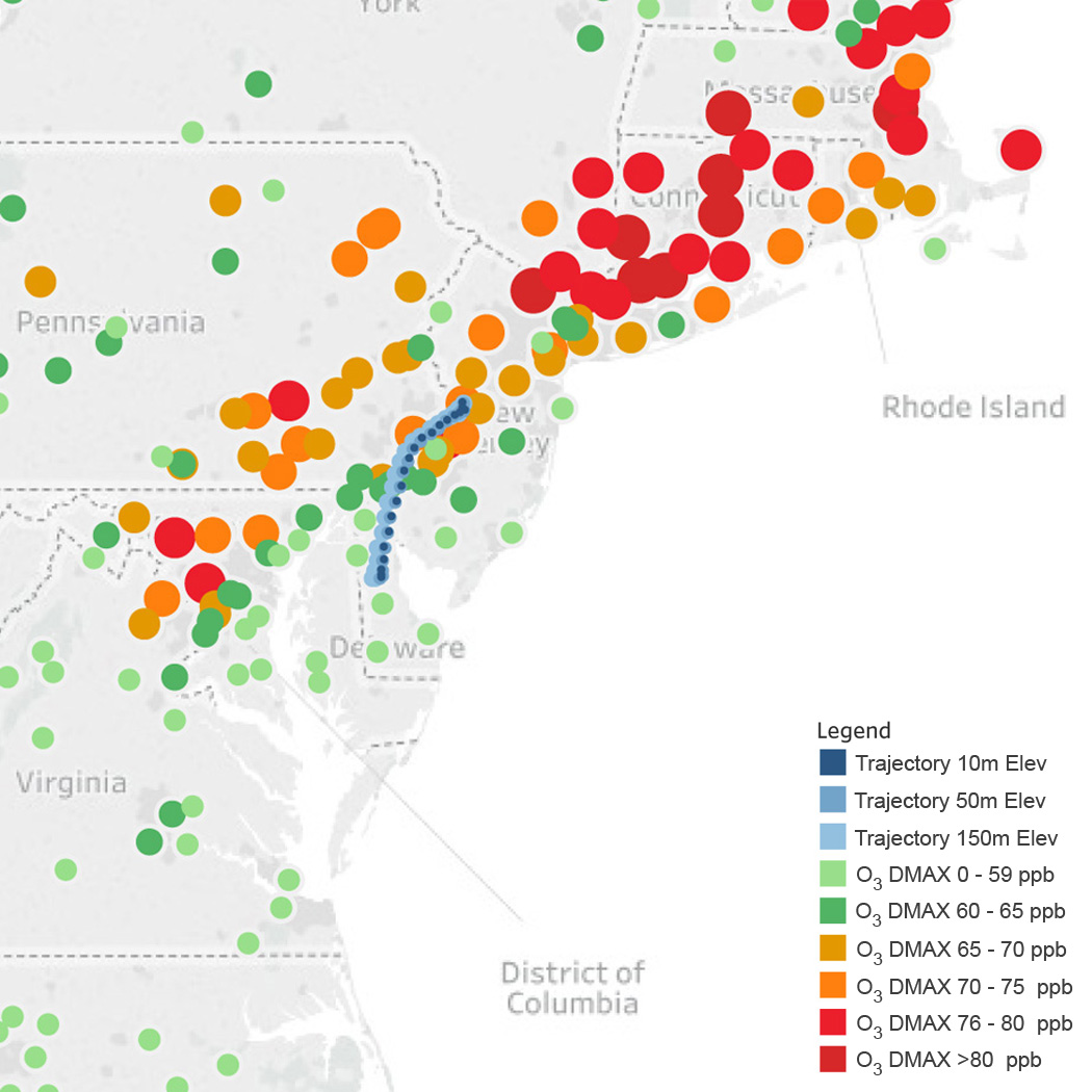
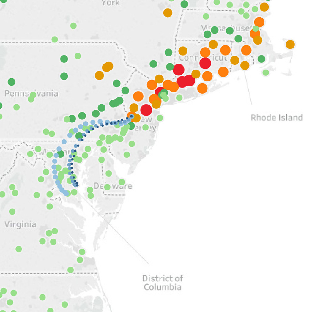
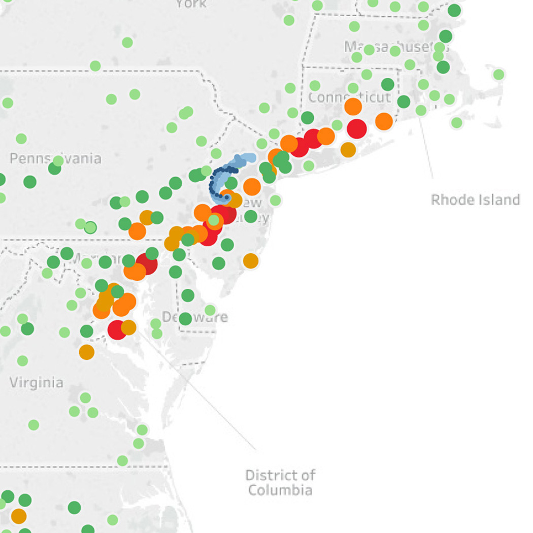
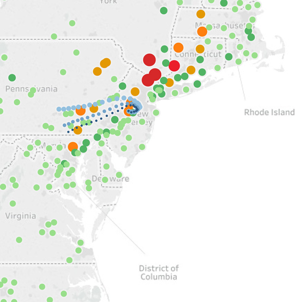
Figure 3-3 shows regional maps with DM8A concentrations at regulatory sites during the eight days when WSP144 reported DM8A concentrations above 70 ppb. The patterns of high O3 concentrations demonstrate the widespread regional nature of elevated DM8A values and show that the patterns varied from episode to episode. On some days (e.g., June 11), the region of elevated O3 concentrations extended from Annapolis, MD to the Connecticut/Rhode Island border along the Mid- Atlantic to Northeast urban corridor, a distance of approximately 550 km. On other days, (e.g., July 29), the region of elevated O3 concentrations was much smaller, extending only from central New Jersey to Connecticut. These patterns mirror the correlation map (Figure 3-1) in that O3 levels measured in central New Jersey were consistently correlated while concentrations measured farther away showed weaker correlation. In short, the episodic patterns of high O3 concentrations were related to emission patterns and synoptic scale weather events and to meteorological parameters, such as ambient temperature, relative humidity, wind speed, and wind direction that affect air mass and pollutant transport.
To better understand the effect of air mass transport on the episodic high regional O3 concentrations, the Hybrid Single Particle Lagrangian Integrated Trajectory model (HYSPLIT; Stein et al., 2015) was run for the eight days. The air masses affecting WSP144 on high O3 days were tracked backward in time over 24-hour periods. The trajectories show the air mass movement pattern and distance covered over the 24-hour period preceding its arrival at the measurement site, recognizing the simulated 24-hour air masses would have traveled and evolved over even longer times and distances. These 24-hour back trajectories were based on 10-, 50-, and 150-m starting elevation heights and were driven by North American Regional Reanalysis meteorological conditions. The trajectories are shown in Figure 3-3, while the distances between the origin of the trajectory and WSP144 are shown in Table 3-2. 5 The two distance categories are the straight line distance and the curved path distance. 6
All 24-hour trajectories, except for two, pass through upwind states outside New Jersey. The 24-hour trajectory for the May 8 episode tracks back to the New Jersey coastline, while the September 2 episode tracks back within New Jersey. Incidentally, the September 2 episode not only had the shortest back trajectory distances for both the straight line and curved path measurements, but also had an origin located to the northeast of WSP144. This was the only trajectory that did not arrive from the southwesterly direction and was the only one of the eight that did not have an average 24-hour back trajectory straight line distance in excess of 100 km, suggesting that O3 transport was important in all but this one episode.
In conclusion, seasonal O3 measurements at WSP144 were highly correlated with O3 measurements from regulatory monitors in the surrounding region. The correlation patterns were also evident for high O3 episodes when the DM8A values exceeded 70 ppb. These analyses, in addition to the site’s central location within the region and fulfillment of CASTNET siting criteria, indicate that WSP144 provides regionally representative measurements. HYSPLIT model runs for eight elevated O3 days in 2015 show that air masses were transported to WSP144 most frequently from upwind states from a southwesterly direction. The HYSPLIT model runs support the CAMx modeling results that indicate both upwind state and in-state contributions affect O3 concentrations measured at WSP144. More research and analysis are needed to understand the effects of meteorology and local and transported emissions for all observed elevated O3 events.
Figure 3-3 Daily Maximum O3 Concentrations Measured at WSP144 and Nearby Regulatory Sites with HYSPLIT 24-hour Back Trajectories when WSP144 Exceeded 70 ppb
1 For a list of the areas that have been designated as nonattainment, see the EPA Green Book https://www.epa.gov/green-book. To review O3 trends at these and other monitors, view https://www.epa.gov/air-trends/air-quality-design-values.
2 Clean Air Act section 110(a)(2)(D)(i)(I).
3 For the CSAPR update, the modeled 2017 base case design values were based on a projected scenario where a number of EGUs (including several in Pennsylvania) were modeled to have particularly high NOx emissions because they were not using selective catalytic reduction (SCR) controls. As a result of the final CSAPR update and the Pennsylvania reasonably achievable control technology rule, both of which are effective in 2017, NOx control regulations are expected to result in these units operating SCR controls in 2017.
4 A linear regression equation was fit to all sites within 250 km of WSP144, and a formula for the expected coefficient of determination was calculated as a function of distance, i.e., y = -(0.00213238)*(distance) + 1.
5 The distances between the receptor and the origin of the air mass 24 hours prior were measured and averaged over the three starting elevations for each date.
6 The straight line distance is the “as the crow flies” distance between the monitor and the location of the start of the trajectory; straight line distance was used by Camalier et al. (2007) as an important factor to understand O3 transport events. The curved path distance is the sum of the distance covered by the air mass over the 24-hour time period.
Nitrogen Pollutant Concentrations
Weekly average concentrations of nitric acid, particulate nitrate, and particulate ammonium were measured using 3-stage filter packs at 95 CASTNET monitoring stations during 2015. Box pots are used to illustrate trends in annual total nitrate (nitric acid plus nitrate) and ammonium concentrations aggregated over 34 eastern and 16 western reference sites. The nitrogen pollutants measured at the eastern reference sites declined over the 26-year period from 1990 through 2015. Mean annual concentrations of total nitrate were reduced by 46 percent from 1990 through 2015. Ammonium concentrations declined by 57 percent. Total nitrate and ammonium concentrations measured at the western reference sites were reduced by 30 percent and 23 percent, respectively, over the 20-year period 1996 through 2015.
Annual mean concentrations of total NO3- (HNO3 + NO3-) and NH4+ for 2015 are presented in two maps in this chapter. Additional maps of 2015 quarterly mean concentrations are provided in CASTNET quarterly data reports (Amec Foster Wheeler, 2015a; 2015b; 2016a; 2016b; 2016c). Trends in annual mean concentrations over the 26-year period (1990 through 2015) were derived from measurements from the eastern reference sites and for the period 1996 through 2015 from data measured at western reference sites. See Appendix A for the designated reference sites.
Total Nitrate Concentrations
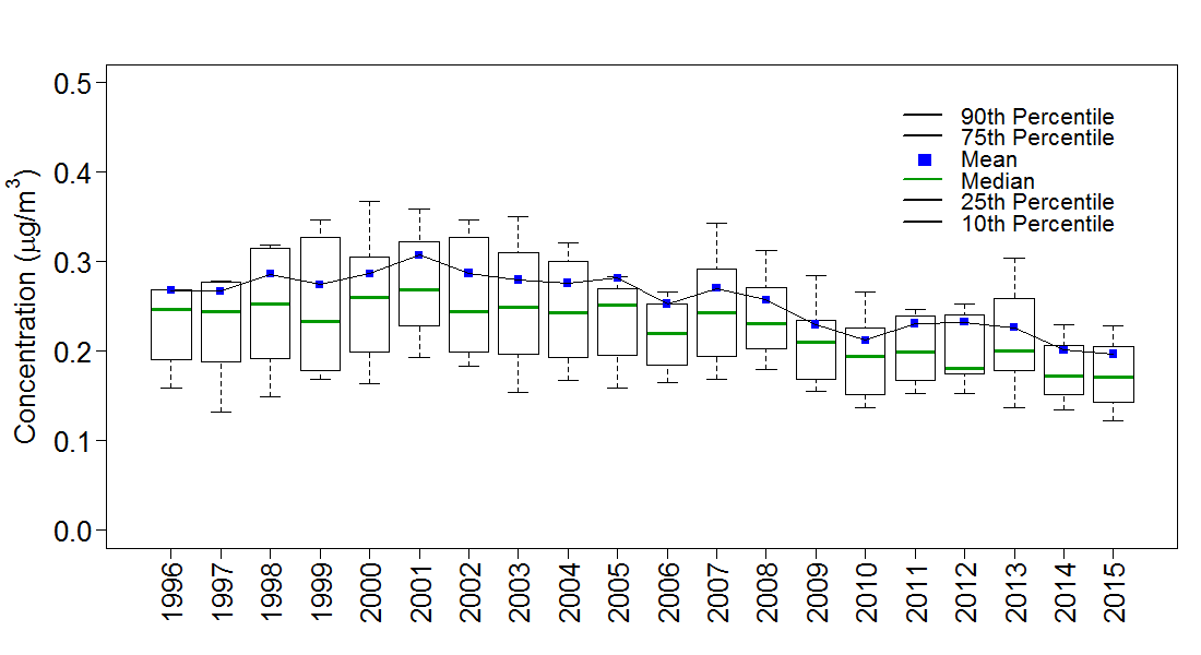
Mean total NO3- concentrations measured in 2015 are presented in the map in Figure 4-1. To illustrate trends, Figure 4-2 provides box plots of total NO3- levels for the eastern and western reference sites through 2015. Each box presents the mean and median concentrations and the 10th, 25th, 75th, and 90th percentiles for that year. The data shown on the right side of the figure were aggregated from the eastern reference sites. The data show no trend in mean concentrations until 2000 when total NO3- levels began to decline in response to NOx emission controls. Total NO3- levels measured at the eastern reference sites were reduced by 50 percent from a mean value of 3.1 micrograms per cubic meter (μg/m 3 ) of air in 2000 to a mean value of 1.6 μg/m 3 in 2015. Over the history of the network, 3-year mean levels declined from 3.0 μg/m 3 for 1990–1992 to 1.6 μg/m 3 for 2013–2015, producing a 46 percent reduction in total NO3-.
The left side of Figure 4-2 shows data aggregated from the western reference sites. Total NO3- levels declined from 1.1 μg/m 3 to 0.7 μg/m 3 from 2000 through 2015, a 36 percent reduction. The 3-year mean total NO3- concentration for 2013–2015 was 30 percent lower than the corresponding 1996–1998 level. The 3-year mean concentration was 1.0 μg/m 3 for 1996–1998 and 0.7 μg/m 3 for 2013–2015.
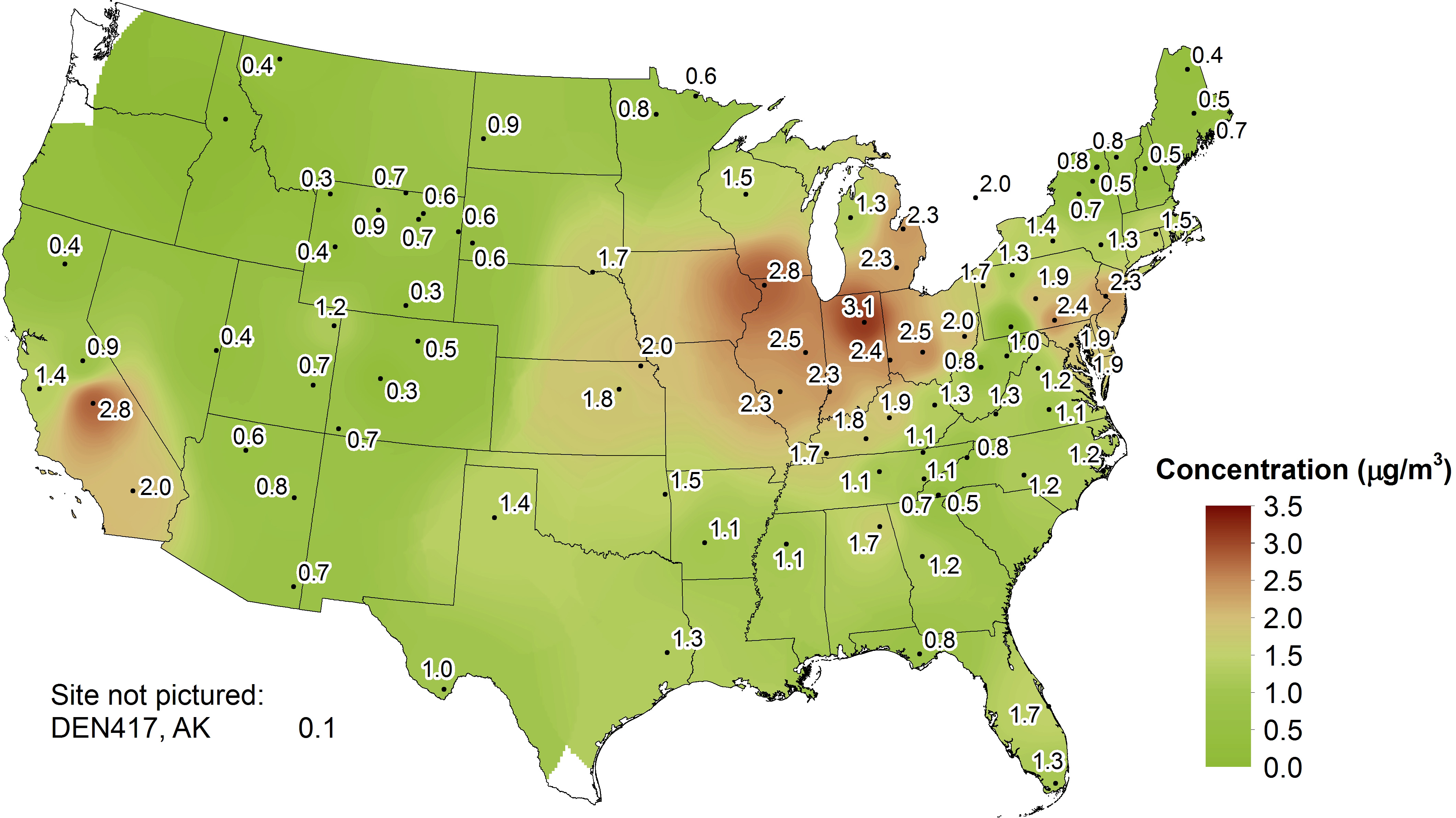
Total nitrate concentrations measured at the eastern reference sites declined by 46 percent since 1990. Total nitrate levels measured at the western reference sites were reduced by 30 percent since 1996. Total nitrate concentrations measured at the eastern reference sites were two to three times higher than concentrations measured at western reference sites.
Figure 4-3 illustrates the trend in NOx emissions from regulated EGUs operating from 1990 through 2015 in six eastern states: Illinois, Indiana, Kentucky, Ohio, Pennsylvania, and West Virginia. The 26- year decline in aggregated EGU emissions in these states was 82 percent.
Figure 4-2 Trends in Annual Mean Total NO3- Concentrations
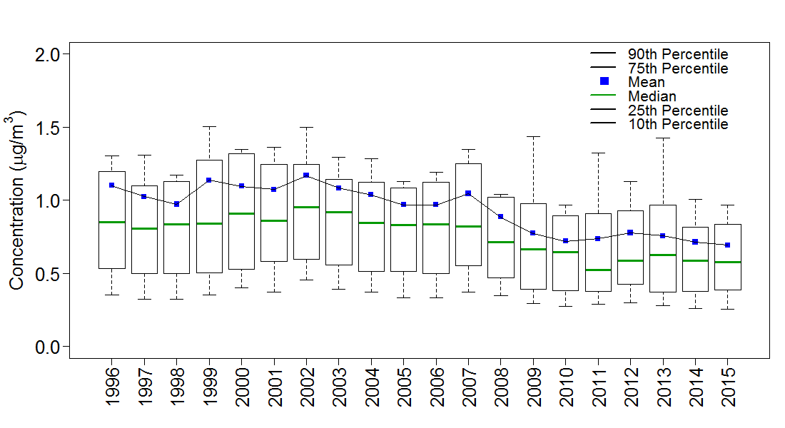
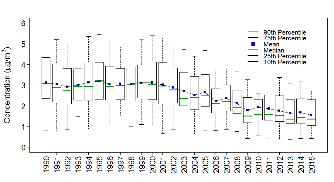
Figure 4-3 illustrates the trend in NOx emissions from regulated EGUs operating from 1990 through 2015 in six eastern states: Illinois, Indiana, Kentucky, Ohio, Pennsylvania, and West Virginia. The 26- year decline in aggregated EGU emissions in these states was 82 percent.
Figure 4-3 Trend in Annual Composite NOx Emissions from Regulated EGUs Operating in Illinois, Indiana, Kentucky, Ohio, Pennsylvania, and West Virginia
 Download Figure
Particulate Ammonium Concentrations
A map of 2015 mean particulate NH4+ concentrations is provided in Figure 4-4. Figure 4-5 shows box plots of NH4+ concentrations. The trend diagram for the eastern reference sites (rightside) shows a reduction in mean NH4+ levels from 1990–1992 to 2013–2015. The 1990–1992 mean concentration was 1.8 μg/m 3 , and the 2013–2015 value was 0.8 μg/m 3 , a 57 percent decline. Similar to total NO3-, the eastern NH4+ concentrations began to decline in 2000 and have been reduced from 1.6 μg/m 3 in 2000 to 0.6 μg/m 3 in 2015. The western reference sites show a decline from 0.3 μg/m 3 in 1996–1998 to 0.2 μg/m 3 in 2013–2015, a 23 percent reduction.
Quality Assurance Program Results
Precision of Filter Pack Measurements
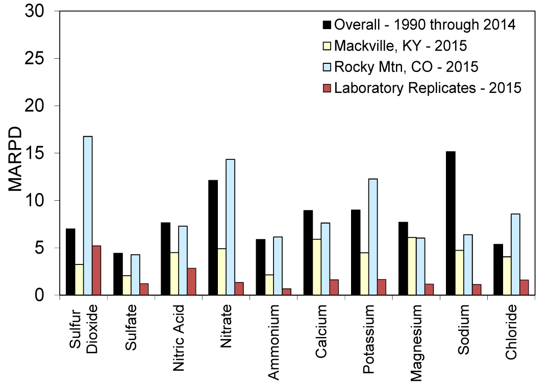
Historical (1990 through 2014) mean absolute relative percent difference (MARPD) data for all 11 co-located site pairs operated over the history of the network are provided in the bar chart in Figure 4-a. The 2015 data for the current co-located sites at MCK131/231 and ROM406/206 are also provided. The precision criterion is a MARPD of 20 percent. Historical and 2015 measurements met the criterion for each analyte.
Figure 4-a Historical and 2015 Precision Results for Atmospheric Concentrations and Laboratory Replicate Samples
 Download Figure
The 2015 analytical precision results for 10 measurements are presented in Figure 4-a. The results were based on analysis of 5 percent of the samples that were randomly selected for replication in each batch. The results of in-run replicate analyses were compared with the original concentration results. The laboratory precision data met the 20 percent measurement criterion.
Data Completeness
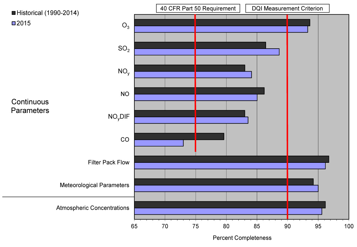
Completeness is defined as the percentage of valid data points obtained from a measurement system relative to total possible data points. The CASTNET measurement criterion for completeness requires a minimum completeness of 90 percent for every measurement for each quarter.
Figure 4-b Historical and 2015 Percent Completeness of Measurements (black bars are 1990–2014 for long-term data and 2013–2014 for trace-level gas data)
 Download Figure
The historical results and the results for 2015 are given in Figure 4-b. Historical results for trace-level gas measurements represent data from 2013–2014. The completeness criterion was met for atmospheric (filter pack) and O3 concentrations, filter pack flow, and meteorological measurements. Completeness of trace-level gas measurements (Chapter 7) met the completeness requirements of 40 CFR Part 50 (EPA, 2015b), except for CO. The substandard completeness for CO was caused by calibration drift in August and sample pump failure and replacement in November.
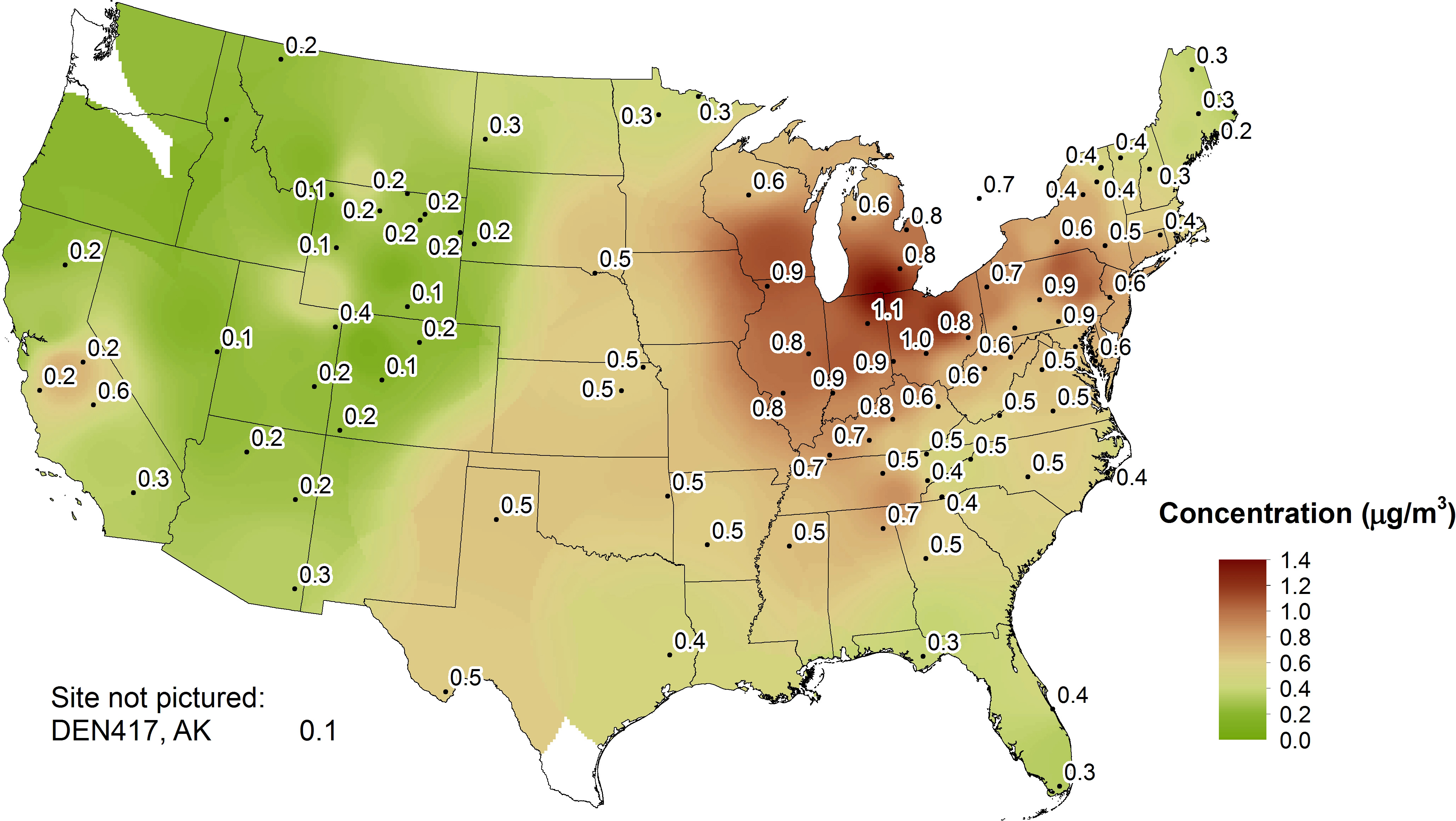
Figure 4-5 Trends in Annual Mean NH4+ Concentrations
Chapter 5: Update on the Ammonia Monitoring Network
The Ammonia Monitoring Network (AMoN) operates passive ammonia samplers at 103 locations, 68 of which are located at CASTNET sites. AMoN is managed by the NADP. The network has been in operation since 2007 and provides information on 2-week integrated ammonia concentrations. Like other NADP networks, the goal of AMoN is to operate a long-term (i.e., for several decades), spatially diverse network with consistent measurements at as many as 300 sites, covering all sensitive ecoregions of the continental United States.
Reduced nitrogen (NH3 + NH4+ ) is an important component to total nitrogen deposition. Wet deposition of NH4+ measured by NTN has been increasing in many areas of the United States over the past 10 years; however, until 2007, gaseous NH3 concentrations were not routinely measured (Li et al., 2016). NH3 is the most prevalent alkaline gas in the atmosphere and is released into the air from a variety of agricultural sources (animal waste, fertilizer application, and agricultural burning), biological sources, gas and oil production and processing, and combustion. Agriculture is by far the largest source, producing approximately 80 percent of gaseous NH3 emissions (EPA National Emissions Inventory, 2014a). Although NH3 has beneficial applications, such as NH3-based fertilizer use, it can have a negative effect on the environment when it reacts with acidic ions such as SO42- and NO3- to 43 form PM2.5, which contributes to negative impacts on human health and visibility degradation. Atmospheric deposition of reduced nitrogen also contributes to eutrophication of sensitive ecosystems, decreases in species diversity, and increases in invasive species.
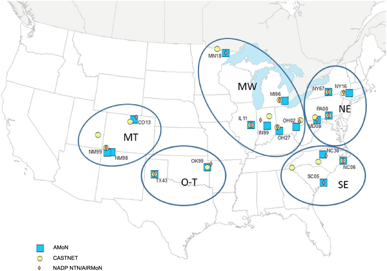
Ambient concentrations of NH3 have shown little to no decrease despite significant reductions in NOx emissions nationwide. Butler et al. (2016) showed that NH3 concentrations measured at 18 of the longest operating AMoN sites have increased over large regions of the United States. Figure 5-1 shows the 18 AMoN sites that have been operating since 2010, with most sites operating since 2007. The sites were allocated into regions with similar seasonal trends and ambient concentrations. The regions and sites are listed in Table 5-1. The map also shows nearby CASTNET and wet deposition sites (NTN or AIRMoN).
Laurel Hill State Park, PA (LRL117)
Table 5-1 Long-term AMoN Sites Located within Five Study Regions
| Region | AMoN Site | AMoN Start Date | Nearby CASTNET Site | Nearby NTN or AIRMoN Site |
|---|---|---|---|---|
| Northeast (NE) | NY16 | 10/2009 | CAT175, NY | NY68 |
| NY67 | 10/2007 | CTH110, NY | NY67 | |
| PA00 | 10/2009 | ARE128, PA | PA00 | |
| MD08 | 08/2010 | LRL117, PA | MD08 | |
| Midwest (MW) | IL11 | 10/2007 | BVL130, IL | IL11 |
| IN99 | 10/2007 | SAL133, IN | IN41 | |
| MI96 | 10/2007 | ANA115, MI | MI52 | |
| MN18 | 10/2007 | VOY413, MN | MN18 | |
| OH02 | 10/2007 | QAK172, OH | OH49 | |
| OH27 | 10/2007 | OXF122, OH | OH09 | |
| Southeast (SE) | NC06 | 04/2010 | BFT142, NC | NC06 |
| NC30 | 06/2008 | CND125, NC | NC36 | |
| SC05 | 10/2007 | COW137, NC | SC05 | |
| Mountain West (MT) | CO13 | 10/2007 | ROM406, CO | CO22 |
| NM98 | 10/2007 | MEV405, CO | CO99 | |
| NM99 | 10/2007 | CAN407, UT | CO99 | |
| Oklahoma-Texas (O-T) | OK99 | 10/2007 | CHE185, OK | AR27 |
| TX43 | 10/2007 | PAL190, TX | TX43 |
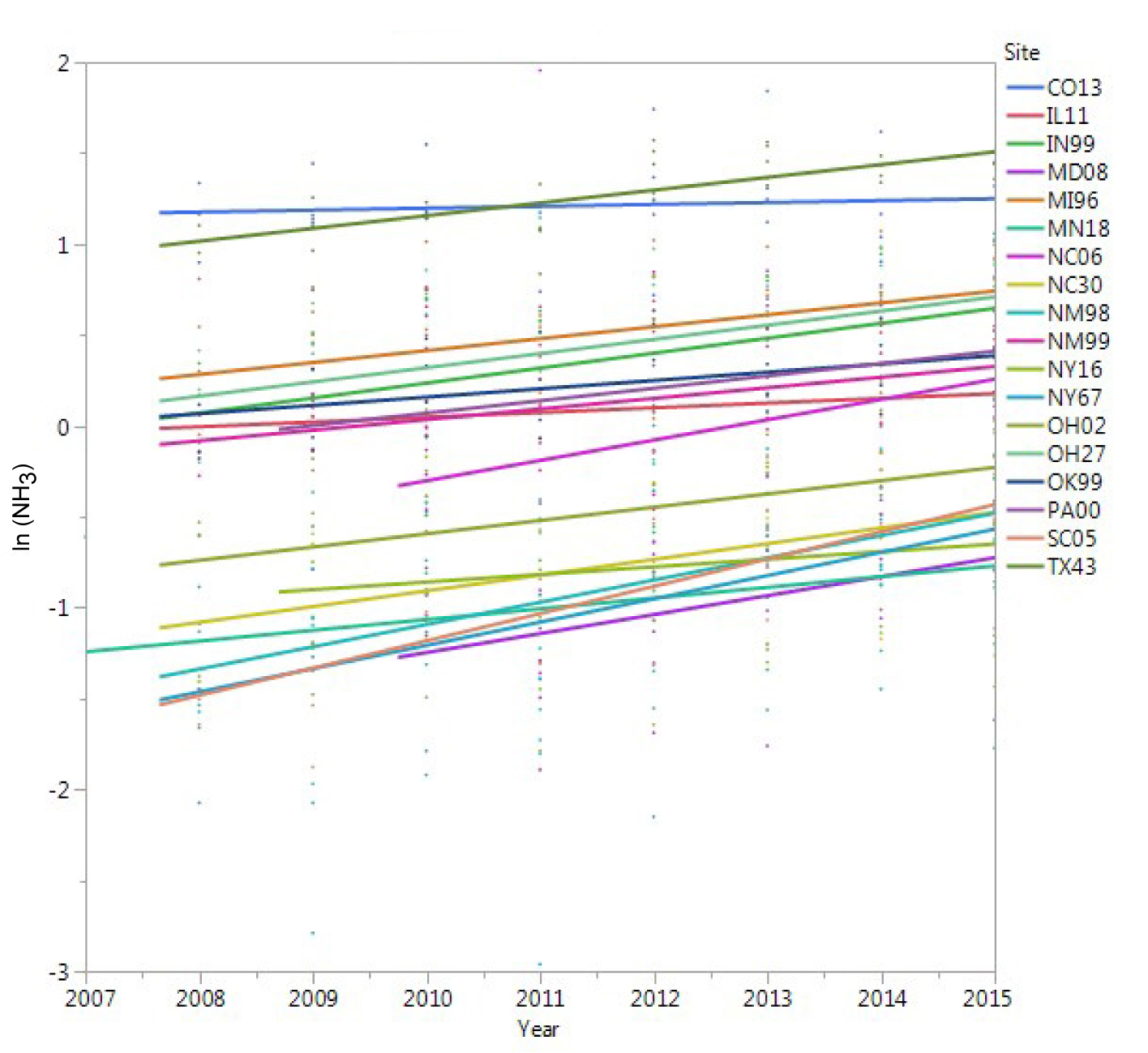
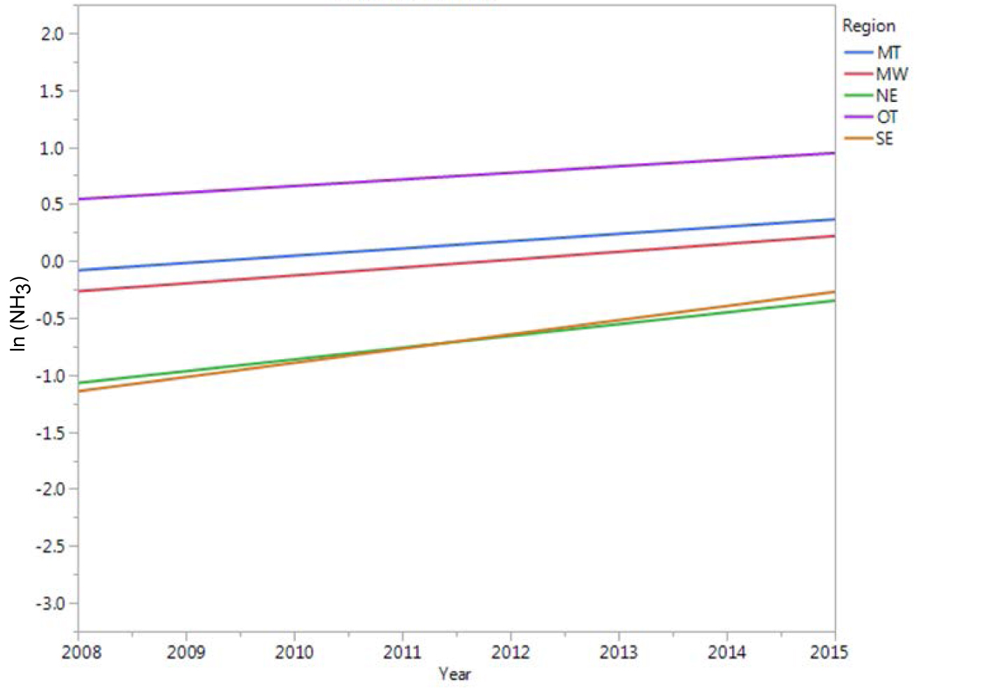
The average increases in NH3 concentrations for the 18 sites over a 9-year period was 7 percent per year (95 percent confidence interval). Figures 5-2 and 5-3 show regressions based on the natural logarithm (ln) of observed annual NH3 concentrations (2007 through 2015) for (a) the 18 long-term AMoN sites and (b) the 5 regions. Points are the individual annual concentrations from each site used in the analysis. There was a similar increase in NH4+ in precipitation at NTN and AIRMoN sites over the same period. Butler et al. (2016) found an increase of 5 percent per year (95 percent confidence interval)in NH4+ in precipitation at the co-located or nearby wet deposition sites. Significant reductions in CASTNET-measured ambient total NO3- concentrations, which follow trends in NOx emissions, do not translate into reductions in total nitrogen because of increases in ambient NH3.
Figure 5-2 Regression of Natural Log (In) of NH3 from 18 Individual AMoN Sites
 Download Figure
Source: Butler et al. (2016)
Figure 5-3 Regression of Natural Log (In) of NH3 from Regional Aggregates
 Download Figure
Source: Butler et al. (2016)
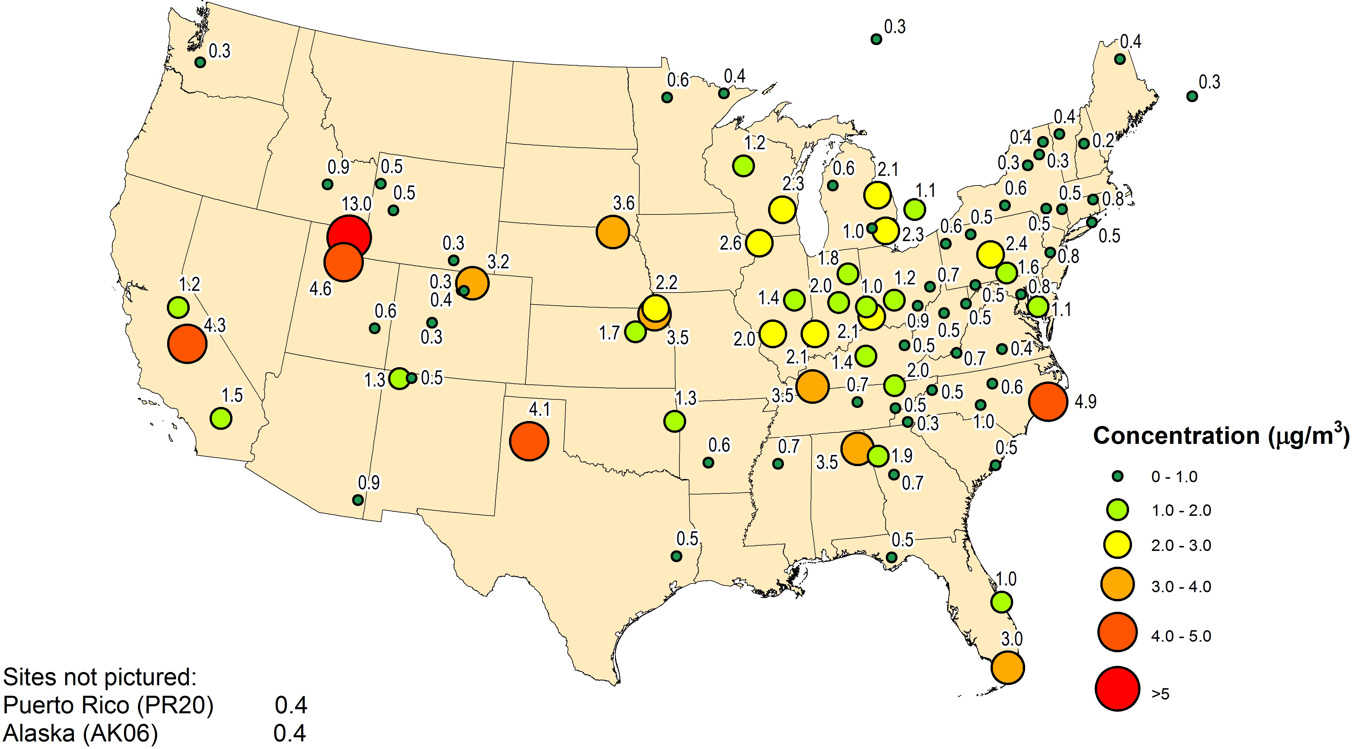
Average annual NH3 concentrations for 2015 for the 66 sites that met completeness requirements are mapped in Figure 5-4 and show a wide range of concentrations from a low of 0.3 μg/m 3 at several northern sites to a high of 13.0 μg/m 3 in northern Utah (UT01), which measured the highest annual average. The Utah monitoring site is located on a Utah State University research farm, and small quantities of livestock are often present (Martin and Baasandorj, 2016). The farm is situated in the Cache Valley, an area with frequent stagnant weather. The next highest concentrations in the West ranged from 3.2 to 4.6 μg/m 3 at six sites west of the Mississippi River. The highest concentration east of the Mississippi was observed at Beaufort, NC (NC06) with a mean concentration of 4.9 μg/m 3 . High local NH3 concentrations are largely influenced by agricultural operations (e.g., hog and cattle feeding and waste and crop fertilization and production).
Chapter 6: Sulfur Pollutant Concentrations
Weekly average concentrations of sulfur dioxide and particulate sulfate were measured using 3-stage filter packs at 95 CASTNET monitoring stations during 2015. Annual sulfur dioxide and sulfate concentrations were aggregated over 34 eastern and 16 western reference sites in order to estimate trends, which are depicted using box plots. The sulfur dioxide pollutants measured at the eastern reference sites declined by 83 percent over the 26-year period from 1990 through 2015. Particulate sulfate concentrations were reduced by 66 percent. Measured concentrations of sulfur dioxide and sulfate have decreased steadily since 2005. Sulfur dioxide and sulfate concentrations measured at the western reference sites have decreased by 47 and 25 percent, respectively, over the 20-year period 1996 through 2015.
Annual mean concentrations of SO2 and SO42- for 2015 are presented in this chapter. Additional maps 24 of 2015 quarterly mean concentrations are provided in CASTNET quarterly data reports (Amec Foster Wheeler, 2015a; 2015b; 2016a; 2016b; 2016c). Trends in annual mean concentrations over the 26-year period (1990 through 2015) were derived from measurements from the eastern reference sites and for the period 1996 through 2015 from data measured at western reference sites. See Appendix A for descriptions of the designated reference sites.
Sulfur Dioxide Concentrations
During review of concentrations measured from May through December 2015, it was determined that a positive bias for SO2 concentrations measured by the impregnated cellulose filters had been introduced through the use of a potassium carbonate reagent from a new vendor. Data analysis and field testing showed that the bias was present following filter exposure to ambient air and had the largest effect on low concentration samples. Samples collected during the May through December 2015 period were adjusted by decreasing all concentrations by 0.16 micrograms per milliliter before total microgram and atmospheric concentration calculations were applied. The adjustment was determined by reviewing the 5th, 10th, and 25th percentiles of the affected time period compared with unaffected (prior) years. All percentiles gave approximately the same increase during the affected time period, showing this to be a positive, constant bias as opposed to a percentage increase. Affected data were flagged to indicate the adjustment was made.
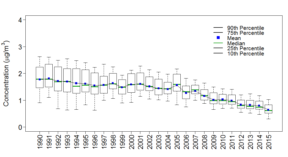
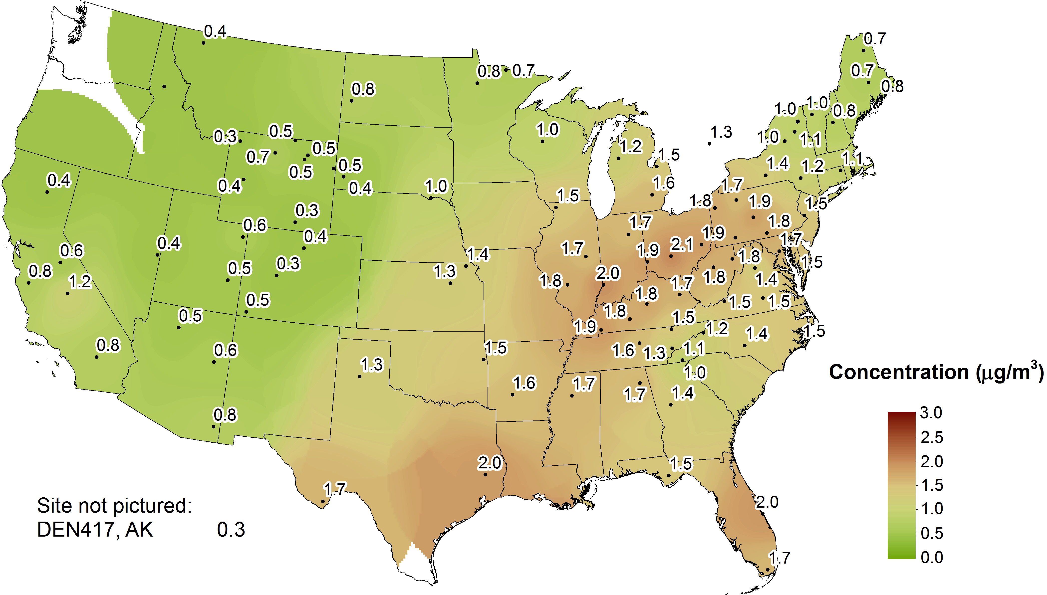
Annual mean SO2 concentrations are shown in Figure 6-1 for 2015. Annual mean concentrations were highest in the Midwest and East near and downwind of the Ohio River. Box plots of annual SO2 concentrations aggregated over the eastern reference sites from 1990 through 2015 (right side) and the western reference sites from 1996 through 2015 (left side) are depicted in Figure 6-2. The y-axes on the eastern and western plots have different scales because concentrations measured at the western sites were much lower than those measured at the eastern sites. Three-year mean concentrations for the eastern reference sites for 1990–1992 and 2013–2015 were 8.8 μg/m 3 and 1.4 μg/m 3, respectively. This change constitutes an 83 percent reduction in 3-year mean SO2 concentrations between the two periods. The 2015 mean level of 1.2 μg/m 3 was the lowest concentration measured by the eastern reference sites in the history of the network and represents a significant decline from the 2005 mean concentration of 6.0 μg/m 3.
The box plots for the western reference sites indicate a decline in annual mean SO2 concentrations aggregated over the 16 sites. Three-year mean SO2 concentrations for 1996–1998 and 2013–2015 were 0.6 μg/m 3 and 0.3 μg/m 3, respectively. This change constitutes a 47 percent reduction in 3-year mean SO2 concentrations at the western reference sites over the 20 years.
The 2015 average sulfur dioxide concentration for the eastern reference sites was 1.2 μg/m 3 . The eastern sulfur dioxide data show a substantive decline since 1997. The reduction (83 percent) in sulfur dioxide concentrations over the period 1990 through 2015 is consistent with the reduction (86 percent) in sulfur dioxide emissions from EGUs operating in the eastern United States, suggesting an approximately linear relationship between concentrations and emissions.
Figure 6-2 Trends in Annual Mean SO2 Concentrations
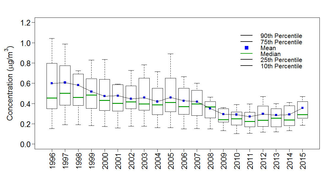
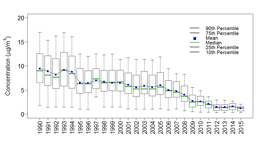
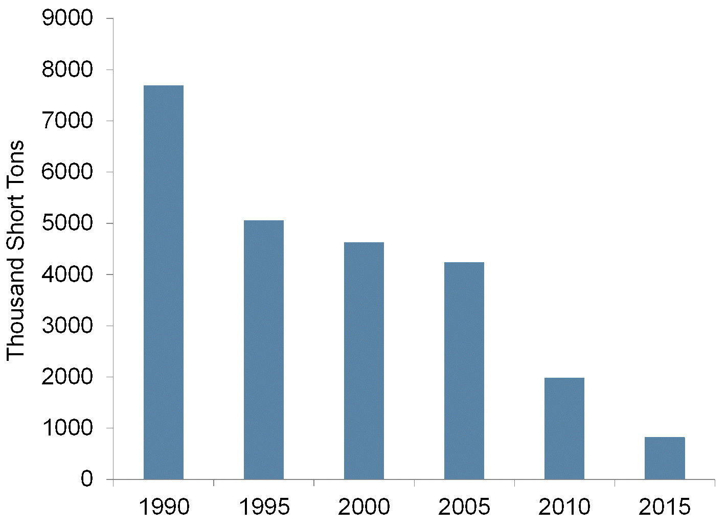
Figure 6-3 Trend in Annual Composite SO2 Emissions from Regulated EGUs Operating in Illinois, Indiana, Kentucky, Ohio, Pennsylvania, and West Virginia
 Download Figure
Figure 6-3 illustrates the trend in SO2 emissions from regulated EGUs operating from 1990 through 2015 in six eastern states: Illinois, Indiana, Kentucky, Ohio, Pennsylvania, and West Virginia. The 26- year decline in aggregated EGU emissions in these states was 89 percent.
Particulate Sulfate Concentrations
Figure 6-4 shows a map of 2015 annual mean particulate SO2 concentrations. Figure 6-5 provides 4 box plot of annual SO2 concentrations from the eastern reference sites (right side) and western 4 reference sites. The figure shows a substantial decline in SO2 over the 26 years for the eastern 4 reference sites. Of particular interest, concentrations declined rapidly from 2005 through 2015. The difference between 3-year means from 1990–1992 to 2013–2015 represents a 66 percent reduction in SO2 from 5.4 μg/m 3 to 1.8 μg/m 3, respectively. The 2015 mean SO2 level of 1.6 μg/m 3 for the eastern 44 reference sites was the lowest in the history of the network.
The box plot for the western reference sites are provided on the left side of Figure 6-5. The data show a 25 percent reduction in annual mean SO2 concentrations aggregated over the 16 sites with 1996–1998 and 2013–2015 concentrations of 0.8 μg/m 3 and 0.6 μg/m 3, respectively.
The 2015 average sulfate concentration for the eastern reference sites was 1.6 μg/m 3 , the lowest level in the history of the network. The eastern sulfate data show a substantive decline since 2005. Sulfate concentrations declined more slowly than sulfur dioxide concentrations at the eastern reference sites. Western sulfate concentrations were lower and decreased at a slower rate than concentrations measured at the eastern sites.
Sumatra, FL (SUM156)
Chapter 7: Continuous Trace-level Gas Concentrations
Continuous, trace-level, gaseous, air quality monitors were run at eight CASTNET sites during 2015. EPA operated six of the monitors, and NPS operated two. The measurements at these sites were performed to (1) provide data to understand atmospheric processes such as ozone and fine particulate matter formation, (2) generate data for regional model input and evaluation, and (3) support EPA NCore monitoring. Total reactive oxides of nitrogen were measured at all eight sites, sulfur dioxide at four sites, and carbon monoxide at two sites. Total reactive oxides of nitrogen concentrations were highest at the Beltsville, MD site and lowest at the high-elevation, mountainous sites.
Continuous trace-level gas analyzers were deployed at six EPA and two NPS CASTNET sites during 2015. NO/NOy measurements were also taken by other federal, tribal, and state agencies at CASTNET or nearby sites in Maine, North Dakota, Oklahoma, and South Dakota. Table 7-1 lists the site locations, start dates, and the trace-level gas parameters measured at each CASTNET site. These data were sampled continuously and archived as 1-hour values.
Table 7-1 Continuous, Trace-level Gas Monitoring Stations Operated at CASTNET Sites during 2015
| Site Location | Start Dates | Measurements |
|---|---|---|
| Beltsville, MD (BEL116) | March 2005 | NO/NOy and SO2 |
| Mammoth Cave National Park, KY (MAC426)* | May 2009 | NO/NOy, SO2, and CO |
| Bondville, IL (BVL130) | July 2012 | NO/NOy, SO2, and CO |
| Huntington Wildlife Forest, NY (HWF187) | November 2012 | NO/NOy |
| Pinedale, WY (PND165) | May 2013 | NO/NOy |
| Cranberry, NC (PNF126) | October 2013 | NO/NOy |
| Rocky Mountain National Park, CO (ROM206) | October 2013 | NO/NOy |
| Great Smoky Mountains National Park (GRS420)* | November 2014 | NO/NOy and SO2 |
Note: *Operated by NPS
NOy is defined as NOx [NO + nitrogen dioxide (NO2)] plus NOz [HNO3, nitrous acid (HONO), peroxyacetyl nitrate, peroxyproyl nitrate, other organic nitrates, and nitrite]. NOy consists of reactive gases that are considered precursors of O3 and PM2.5. NOy is measured by conversion to NO using a thermal catalytic converter and measurement of the NO by chemiluminescence. Continuous SO2 is measured using ultraviolet fluorescence, and CO is measured by gas filter correlation. Data are used to assess the effectiveness of emission reductions, to understand O3 and PM2.5 formation processes, for model input and evaluation, and for comparison with the weekly integrated CASTNET filter pack measurements.
Figure 7-1 provides a map of the CASTNET continuous trace-level gas monitoring locations. All EPA sites were operated according to the CASTNET QAPP Appendix 11, “Procuring, Installing, and Operating NCore Air Monitoring Equipment at CASTNET Sites” (Amec Foster Wheeler, 2014). NPS sites were operated according to their QA protocols. The CASTNET QAPP and all related appendices can be accessed at https://java.epa.gov/castnet/documents.do.

Rocky Mountain National Park, CO (ROM206)
Quality Assurance Program Results
Continuous Trace-level Gas Concentrations
The precision of continuous trace-level gas concentration measurements was estimated based on the acceptance criteria enumerated in 40 CFR Part 58 Appendix A (EPA, 2013) for NOy (including the criteria pollutant NO2), SO2, and CO. Figure 7-a presents summary statistics of critical criteria measurements at EPA-sponsored trace-level gas monitoring sites collected during 2015. All data associated with QC checks that failed to meet the established criteria were invalidated unless the cause of failure was documented to have no effect on ambient data collection. QC failures for EPA-sponsored sites are addressed in quarterly QA reports, which can be found on the EPA CASTNET website.
Note:
QA program results for NPS-sponsored sites measuring trace-level gas may be accessed at http://www.nature.nps.gov/air/monitoring/network.cfm
Figures 7-2 through 7-4 and Figure 7-6 present 2015 annual average hourly composite diurnal profiles of SO2, NOy, and O3 for BEL116, BVL130, MAC426, and GRS420, respectively. Figures 7-5 and 7-7 through 7-9 show the 2015 annual average hourly composite diurnal profiles of NOy and O3 for HWF187, PNF126, PND165, and ROM206. The profiles in Figures 7-2 through 7-9 were constructed by averaging all values from the same hour for their respective time periods. Different scales were used for y-axes. SO2 and NOy are plotted against the left y-axis, and O3 is plotted against the right y-axis in the eight diagrams. The figures illustrate that differences in geography, terrain, and elevation affect the evolution of photochemically reactive pollutants in the boundary layer.
Table 7-2 Summary of 2015 Minimum and Maximum Values from Diurnal Charts
| Site Location | Site Elevation (meters) | NOy (ppb) | O3 (ppb) | ||
|---|---|---|---|---|---|
| Minimum | Maximum | Minimum | Maximum | ||
| BEL116, MD | 47 | 5.9 | 13.7 | 15 | 42 |
| BVL130, IL | 213 | 3.1 | 5.5 | 20 | 41 |
| MAC426, KY | 243 | 2.3 | 3.5 | 23 | 39 |
| HWF187, NY | 497 | 0.7 | 1.1 | 15 | 35 |
| GRS420, TN | 793 | 1.7 | 2.1 | 32 | 41 |
| PNF126, NC | 1,216 | 0.7 | 1 | 37 | 43 |
| PND165, WY | 2,386 | 0.6 | 0.9 | 42 | 49 |
| ROM206, CO | 2,742 | 0.8 | 1.7 | 43 | 50 |
Continuous Trace-level NOy and Ozone
The minimum and maximum mean composite NOy and O3 concentrations shown in Figures 7-2 through 7-9 are summarized in Table 7-2. The sites are listed in order of elevation. The highest NOy concentrations were measured at BEL116, which has numerous, nearby mobile-source NOx emissions. Low NOy values (less than 2.0 ppb) were recorded at the five rural sites in New York, Tennessee, North Carolina, Wyoming, and Colorado. These rural NOy values are similar to Edgerton et al. (2016) NOy measurements at Coweeta, NC. The eight profiles in Figures 7-2 through 7-9 illustrate the loss of O3 during the late afternoon and nighttime hours and its production during daylight hours. The diurnal change was less pronounced at the six rural sites. The BEL116 site observed the largest nighttime loss and subsequent highest daytime production, an average difference of about 27 ppb of O3 for 2015. The BVL130 data illustrate a typical diurnal relationship between NOy and O3 concentrations with high NOy concentrations associated with vehicular NOx emissions in the morning and evening and elevated O3 concentrations in the afternoon. The data from the rural MAC426 site also show a diurnal evolution with the highest NOy concentrations in the morning and the evening and highest O3 concentrations in the afternoon. The MAC426 data appear similar to measurements made at an urban site.
O3 concentrations were also measured at HWF187, GRS420, PNF126, PND165, and ROM206 during 2015 (Table 7-2). Of these sites, the highest O3 concentration (50 ppb) was measured at ROM206. The concentrations measured at the three sites with the highest elevations show less 24-hour variation than the other five sites because of the absence of nighttime O3 loss/depletion mechanisms near the high-elevation monitors (Talbot et al., 2005). In particular, nighttime dry deposition is small because shallow boundary layers typically do not form at these high-elevation sites and scavenging is diminished because fresh nitric oxide is not available to react with O3. The ROM206 data suggest a large production or transport of NOy around sunset. There are no significant NOx sources in the immediate area. The increase in NOy is likely a result of the transformation of polluted air masses from the Front Range Urban Corridor and the frequent late afternoon upslope flow from the east (Baumann et al., 1997).
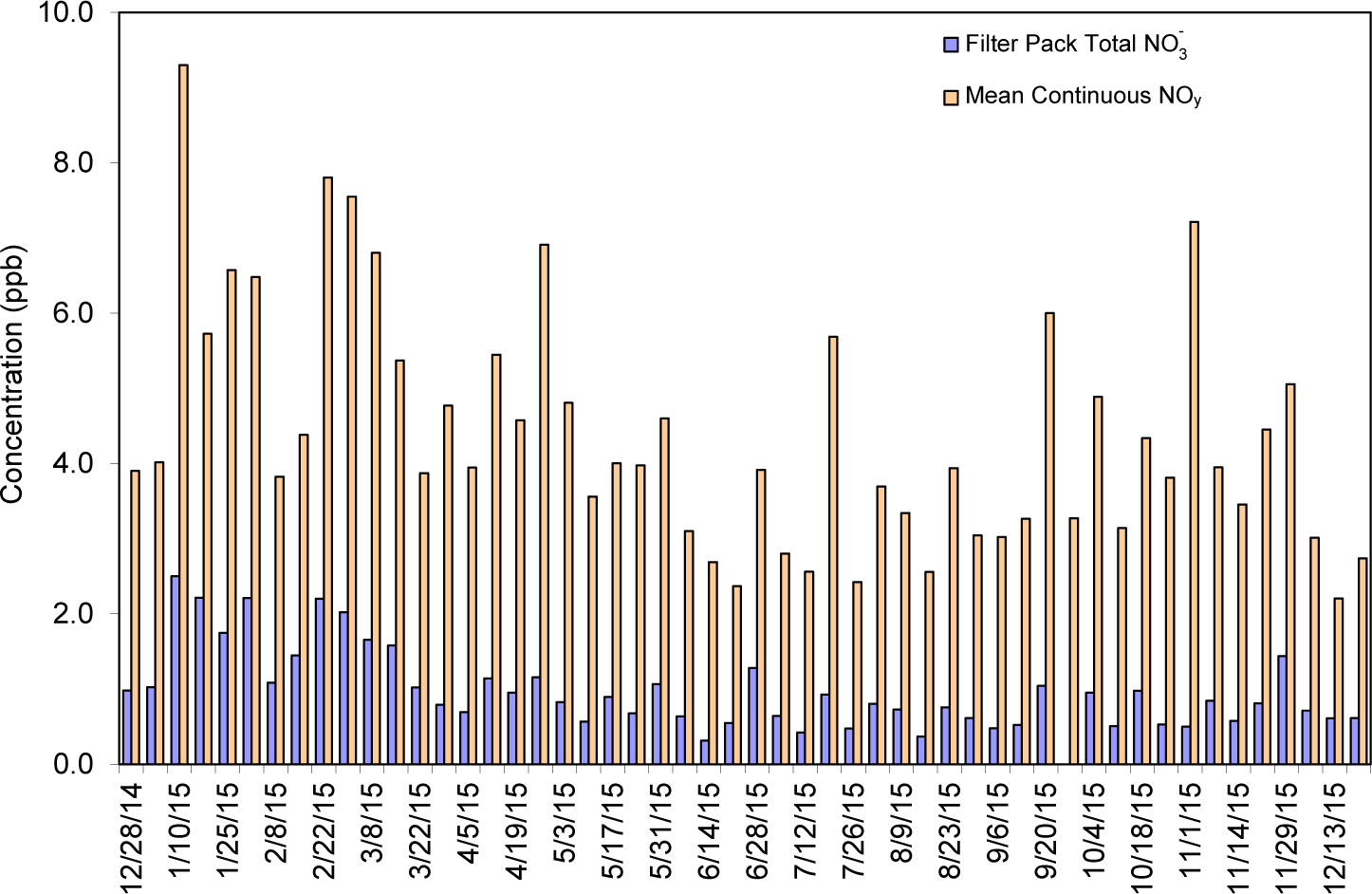
Continuous Trace-level NOy and Filter Pack Total Nitrate Concentrations
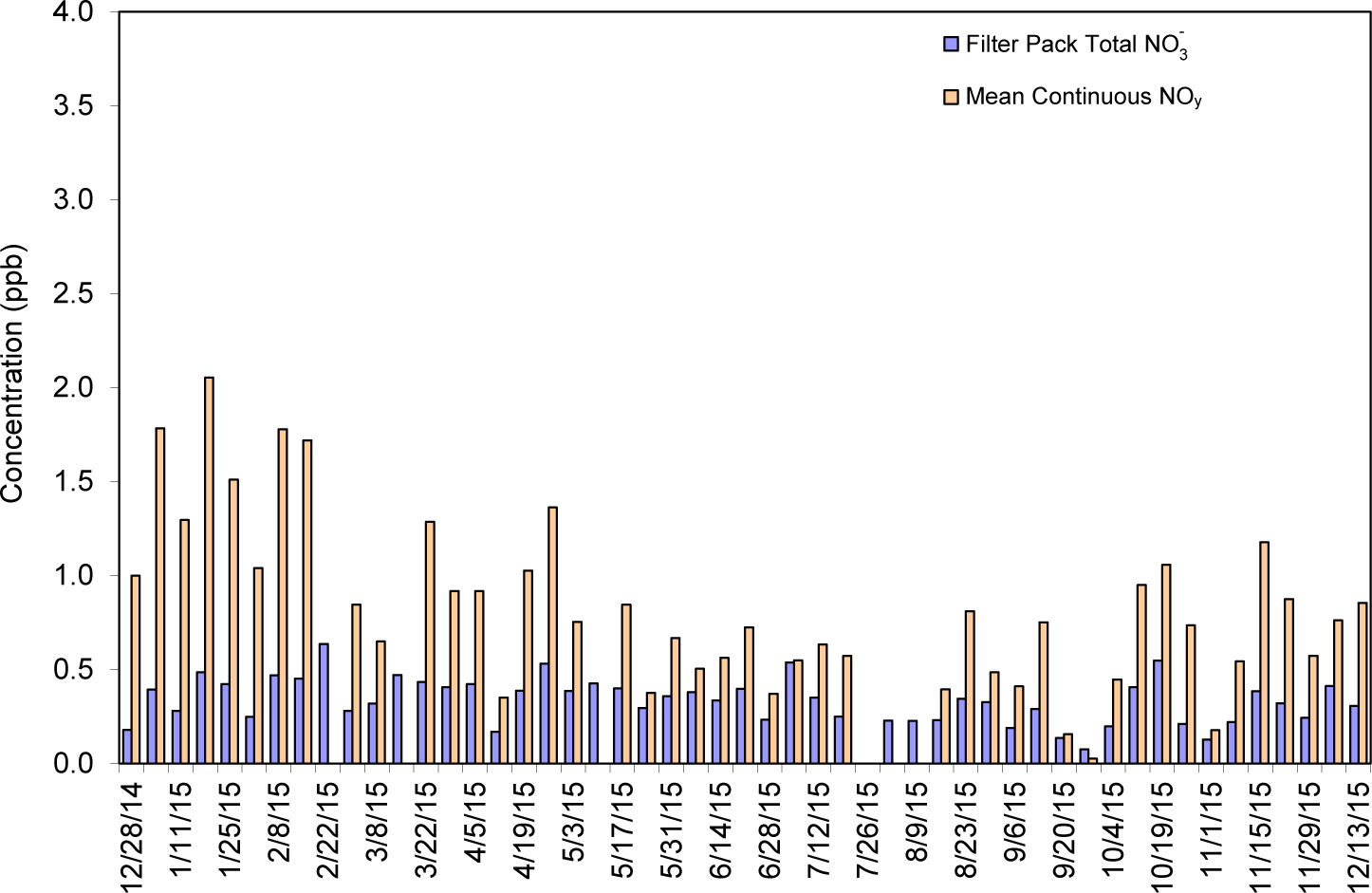
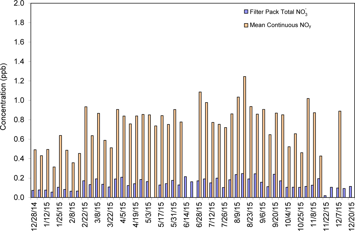
HNO3 and particulate NO3- are measured on CASTNET filter packs, and the sum is reported as total NO3-. Because HNO3 and particulate NO3- are measured as components of NOy, NOy concentrations should always be higher than total NO3- levels (i.e., the ratio of NOy to total NO3- should always be greater than 1.0). A comparison of weekly mean continuous NOy concentrations with filter pack total NO3- levels at BVL130, PNF126, and PND165 for 2015 was used to evaluate the measurements (Figures 7-10 through 7-12). The NOy concentrations were consistently higher than the total NO3- levels, as expected. The results are similar for the other five sites. The weekly total NO3- concentrations, the average weekly NOy levels, and their ratios are listed in Table 7-3. These were calculated as the average of all valid weekly filter pack concentrations, the average of mean NOy values matching the run time of the weekly filter packs, and the average of the ratios calculated for each week. Weekly NOy levels were higher than the weekly total NO3- concentrations with ratios of NOy to total NO3- varying from 2.40 at PNF126 to 10.87 at BEL116. The highest concentration (0.98 ppb) of total NO3- was measured at BVL130.
Bondville, IL (BVL130)
Figure 7-10 Comparison of BVL130, IL Weekly Mean Continuous Trace-level NOy and Filter Pack Total NO3- Concentrations
 Download Figure
Figure 7-11 Comparison of PNF126, NC Weekly Mean Continuous Trace-level NOy and Filter Pack Total NO3- Concentrations
 Download Figure
Figure 7-12 Comparison of PND165, WY NC Weekly Mean Continuous Trace-level NOy and Filter Pack Total NO3- Concentrations
 Download Figure
Table 7-3 Summary of Total NO3- and NOy Measurements for 2015
| Site Location | Total NO3- (ppb) | NOy (ppb) | Ratio |
|---|---|---|---|
| BEL116, MD | 0.76 | 8.01 | 10.87 |
| BVL130, IL | 0.98 | 4.39 | 5.03 |
| MAC426, KY | 0.7 | 2.79 | 4.34 |
| HWF187, NY | 0.21 | 0.94 | 3.58 |
| GRS420, TN | 0.45 | 1.97 | 4.93 |
| PNF126, NC | 0.7 | 0.81 | 2.4 |
| PND165, WY | 0.6 | 0.75 | 5.43 |
| ROM206, CO | 0.8 | 1.2 | 6.59 |
Chapter 8: Deployment and Evaluation of the Monitor for Aerosols and Gases at Beltsville, Maryland
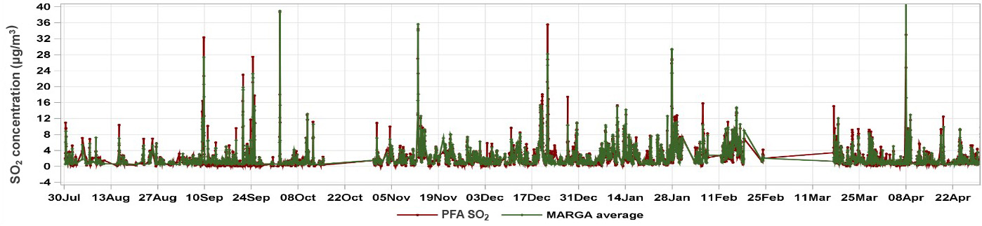
The EPA deployed two separate, co-located Monitor for AeRosols and GAses (MARGA) 1S systems at its CASTNET Beltsville, MD site between August 2014 and May 2015. The measurement campaign produced eight months of valid hourly data for soluble gases (nitric acid, nitrous acid, sulfur dioxide, and ammonia) and particles (nitrate, sulfate, ammonium, calcium, magnesium, potassium, and sodium). The gas and particulate concentration measurements were used to evaluate the performance of the MARGA instrument systems based on (1) filter pack concentration data and (2) data from a conventional pulsed fluorescence sulfur dioxide analyzer. The measurements were also used to intercompare the performance of the two MARGAs.
Comparison of MARGA, Continuous Sulfur Dioxide Analyzer, and CASTNET Filter Pack
To evaluate MARGA measurements, SO2 data from the two MARGA systems were compared with the already operational hourly SO2 measurements from a co-located federal equivalent method pulsed fluorescence SO2 analyzer (PFA). No additional provisions were made to eliminate variables that could lead to measurement differences (i.e., different inlet heights or more frequent calibrations to the analyzer). Thus, the hourly PFA SO2 measurements were compared as a check and not as a performance verification. The agreement of one species (SO2) in the suite of co-located measurements is not a validation of all species measured with the MARGA but does provide additional confidence in overall MARGA performance (Rumsey et al., 2014; McKernan et al., 2011). It is important to note the differences between the two methods. Inlet height for the MARGA was sampled at either 5 or 3 m (inlets were changed midway through the evaluation period); however, this had little effect for SO2 recovery. The PFA inlet was at 10 m. Additionally, the MARGA samples gases semi-continuously every hour via absorption into solution using a wet, rotating denuder with subsequent analysis via on-line ion chromatography. The PFA is an optical emission method for continuous SO2 measurement integrated up to hourly resolution.
The PFA SO2 data required a linear baseline adjustment to correct for drift (evident from calibration data). After the correction, the MARPD between the hourly PFA and the MARGA SO2 concentrations was 32 percent for concentrations exceeding the MARGA method detection limit (MDL) of greater than or equal to 0.05 μg/m 3 . Filtering the data for higher values (greater than or equal to 1.33 μg/m 3 ) improved the MARPD to 22 percent. This analysis indicates that scatter in low-level concentrations is an issue in the co-location and suggests the limit of comparison between the two methods should be set higher than the MARGA MDL. A traditional linear regression was run with the MARGA SO2 concentrations as the independent variable and gave a slope of 0.950 ± 0.007 and y-intercept of 0.022 ± 0.023 with a root mean square error of 1.30 and an R 2 of 0.790. Hourly SO2 concentrations averaged between the two MARGA units and the PFA are shown in Figure 8-1.
Figure 8-1 Time-series of Hourly SO2 Concentrations Based on an Average of Two MARGA Units and PFA from July 30, 2014 through May 4, 2015
 Download Figure
Comparison of Co-located MARGA Units
The sampling campaign with the MARGAs was conducted for eight months between July 30, 2014 and May 4, 2015, with two identical MARGA units (MU1 and MU2) running in the same shelter. The performance metrics of the hourly MARGA measurements are shown in Table 8-1. Sampling during this time resulted in a high percentage of valid data for all species (89–92 percent for MU1 and 87–93 percent for MU2) with an overall time coverage of 82–84 percent valid data from at least one instrument. Overall performance statistics between the co-located MARGA units (Table 8-1) were excellent with MARPD values less than or equal to 15 percent for aerosol species (NH4+ , NO3- , SO42-), 434 values less than or equal to 20 percent for gaseous species (HONO, SO2), and values less than or equal to 25 percent for gaseous HNO3. An exception to this was gaseous NH3 with a MARPD of 39 percent. Linear regression slopes were near an expected value of 1: within ± 5 percent for HNO3, NH4+ , NO3- , and SO42-; within ± 15 percent for HONO; and within ± 18 percent for SO . The slope for NH3 was 30 percent less than 1, indicating a bias between the instruments. Comparison of base cation data, Ca 2+, Na +, Mg 2+, and K + , was affected by low ambient levels nearing detection limits and required blank corrections.
Figure 8-1 Time-series of Hourly SO2 Concentrations Based on an Average of Two MARGA Units and PFA from July 30, 2014 through May 4, 2015
Beltsville, MD (BEL116)
Table 8-1. Statistical Comparisons between Hourly Concentrations (μg/m 3 ) Measured with Co-located MARGA Units from July 30, 2014 through May 4, 2015
| MARPD (%) | Linear Regression | ||||
|---|---|---|---|---|---|
| Species | Overall | N | m | b | R 2 |
| SO2 ŧ ¥ (PFA) | 32 (22) | 4776 | 0.95 | 0.022 | 0.79 |
| HNO3 | 24 | 2979 | 1.039 | 0.011 | 0.748 |
| HONO | 20 | 2975 | 0.857 | 0.088 | 0.695 |
| NH3 | 39 | 3076 | 0.7 | 0.171 | 0.519 |
| SO2 | 16 | 2984 | 0.82 | 0.168 | 0.851 |
| NO3- | 11 | 2895 | 0.952 | 0.014 | 0.98 |
| NH4+ | 15 | 3068 | 0.947 | -0.055 | 0.979 |
| SO42- | 4 | 2654 | 0.973 | 0.106 | 0.955 |
| Ca 2+ | 43 | 3068 | 0.664 | 0.069 | 0.68 |
| Na + | 30 | 3068 | 0.596 | 0.073 | 0.743 |
Note:
Table includes average MARGA hourly SO2 concentrations compared with the PFA hourly SO2 concentrations
ŧ = comparison of values greater than 1.3 μg/m 3 because of baseline correction
¥ = value from average of MU1 and MU2 to compare with PFA SO2
N = number of samples
m = slope
b = intercept
R 2 = coefficient of determination
The MARGA units show more consistent performance in measuring anion aerosols than gases. This was likely due to the higher mobility of gases coupled with high polarity and solubility that led to increased adsorption to the inlet. Results not presented here support that hypothesis.
Integrated MARGA Data and Comparison with Filter Pack Data
To compare the semi-continuous MARGA data with the CASTNET filter pack concentrations, hourly MARGA data were integrated into weekly averages. Only weeks where the MARGA collected at least 100 hours of valid data (i.e., greater than 60 percent) were considered. Time-series plots of the integrated MARGA data, PFA SO2 data, and the CASTNET filter pack data are shown in Figure 8-2. The NH3 concentrations were extrapolated into weekly intervals from AMoN two-week concentrations, which were measured by a passive sampler at the Beltsville site.
Figure 8-2 Time-series of Weekly Concentrations Based on Integrated Averages of the Two MARGA Units, CASTNET Filter Pack, and PFA (SO2 only) from July 30, 2014 through May 4, 2015
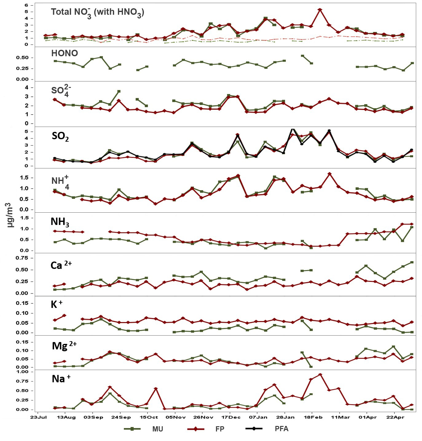 Download Figure
Statistical comparisons were made for each of the species and are shown in Table 8-2. The concentrations measured by the different methods compared very well (i.e., predicted slope within 0.8 to 1.2 and R 2 within 0.8 to 1.2) for SO2 (all measurement methods); total NO3-, which is the sum of HNO3 and NO3- ; NO3- ; and NH4+. Surprisingly, the correlation statistics were not as good for SO42- (m= 0.74; R 2 = 0.61) owing to an observed bias in MARGA concentrations measured from September 12, 2014 to November 5, 2014. Further evaluation is needed to assess if this is a sampling artifact. Interestingly, NH4+ and SO2 also appear to be biased high for the MARGA (and the PFA) during this period.
Table 8-2. Comparison of Concentration (µg/m 3) Statistics for Integrated Weekly Sampling Methods from September 12, 2014 through November 5, 2014
| Species | Dependent Variable | Independent Variable | N | MRPD (%) | MARPD (%) | m (± σ) | b (± σ) | R 2 |
|---|---|---|---|---|---|---|---|---|
| SO2 | PFA | MARGA | 37 | -5 | 11 | 0.933 (0.047) | 0.103 (0.105) | 0.92 |
| SO2 | FP | MARGA | 36 | -5 | 17 | 0.896 (0.072) | 0.160 (0.163) | 0.821 |
| SO2 | FP | PFA | 39 | -5 | 14 | 0.942 (0.058) | 0.089 (0.137) | 0.876 |
| HNO3 | FP | MARGA | 31 | 55 | 55 | 0.915 (0.298) | 0.444 (0.166) | 0.245 |
| NO3- | FP | MARGA | 31 | -24 | 30 | 0.932 (0.065) | -0.154 (0.100) | 0.875 |
| Total NO3- | FP | MARGA | 31 | 12 | 13 | 0.857 (0.060) | 0.404 (0.120) | 0.877 |
| NH3 | FP | MARGA | 31 | 38 | 43 | 0.793 (0.193) | 0.275 (0.096) | 0.368 |
| NH4+ | FP | MARGA | 32 | -8 | 14 | 0.958 (0.083) | -0.044 (0.073) | 0.816 |
| SO2-4 | FP | MARGA | 31 | -17 | 17 | 0.737 (0.110) | 0.193 (0.244) | 0.607 |
| Ca2+ | FP | MARGA | 32 | -54 | 57 | 0.314 (0.060) | 0.102 (0.022) | 0.473 |
| K+ | FP | MARGA | 32 | 90 | 90 | 0.354 (0.118) | 0.051 (0.003) | 0.231 |
| Mg2+ | FP | MARGA | 32 | -12 | 29 | 0.382 (0.077) | 0.026 (0.005) | 0.45 |
| Na+ | FP | MARGA | 32 | 31 | 45 | 1.553 (0.133) | -0.015 (0.025) | 0.821 |
Note:
N = number of samples
m = slope
b = intercept
R 2 = coefficient of determination
σ = standard deviation
The filter pack concentrations for HNO3 were biased higher than the MARGA concentrations [55 percent mean relative percent difference (MRPD)], and there was a low bias of filter pack NO3- concentrations (-24 percent MRPD), which is attributed to the volatilization of ammonium nitrate (NH4NO3) from the Teflon filter to the nylon filter in the CASTNET filter pack setup (Sickles and Shadwick, 2002; Lavery et al., 2009). The MARGA concentrations do not experience any effects due to NH4NO3 volatility as the aerosol is rapidly sampled into the absorbing medium and immediately analyzed (Slanina et al., 2001). A comparison of the total NO3- concentrations (12 percent MRPD) supports this hypothesis. The comparison with NH3 was complicated by the inlet adsorption losses and is being evaluated further.
Chapter 9: Atmospheric Deposition of Nitrogen
CASTNET was designed to provide estimates of the dry deposition of nitrogen and sulfur pollutants across the United States. To assess the status of dry and total deposition for 2015, EPA used NADP’s Total Deposition Hybrid Method to estimate dry deposition. The hybrid method combines measured pollutant concentrations with output from the CMAQ modeling system and uses precipitation chemistry measurements at NADP/NTN sites and precipitation amounts from the Parameter-elevation Regressions on Independent Slopes Model to estimate wet deposition. Total deposition was calculated as the sum of estimated dry and wet deposition.
Gaseous and particulate nitrogen pollutants are deposited to the environment through dry and wet atmospheric processes. A major goal of CASTNET is to estimate the rate of dry deposition of pollutants from the atmosphere to sensitive ecosystems. The NADP TDEP Hybrid Method (EPA, 2015c; Schwede and Lear, 2014) combines monitoring data with output from the CMAQ modeling system (Byun and Schere, 2006) to estimate dry deposition. Air quality measurements were obtained from CASTNET and the Southeastern Aerosol Research and Characterization (SEARCH) Network. The TDEP method gives priority to using measurement data from air quality monitoring sites when available and to CMAQ output in areas where monitoring data are not available. In addition, CMAQ provides modeled data for species that are not routinely measured. The TDEP method and its recent updates are discussed on the TDEP website. See also the NADP Fact Sheet, "Hybrid Approach to Mapping Total Deposition."
TDEP estimates wet deposition using PRISM to develop a continuous grid of precipitation data. PRISM uses terrain elevation, slope, and aspect and climatic measurements to estimate precipitation on a 4-kilometer resolution grid. Pollutant concentrations in precipitation, which were estimated for the PRISM grid, were provided by NADP/NTN. The concentration and precipitation grids were merged in order to estimate pollutant wet deposition rates. Dry and wet deposition fluxes were added to obtain estimates of total deposition, which are presented on the maps in this chapter as kilograms per hectare per year (kg ha-1yr-1).
Figure 9-1 illustrates TDEP estimates of dry fluxes of nitrogen (N) for 2015. The magnitude of the deposition fluxes is illustrated by the shading in the figure legend. A map of total deposition of N for 2015 is given in Figure 9-2. The percentage of total deposition of N due to dry deposition is shown in Figure 9-3. A map of TDEP estimates of total deposition of reduced N species for 2015 is given in Figure 9-4. Figure 9-5 gives the percentage of reduced N species from dry deposition. Dry deposition of N species that are not routinely measured but are estimated by TDEP is shown in the map in Figure 9-6. The percentage of total deposition of N that is not measured directly but is calculated by TDEP is shown in Figure 9-7. Annual gross deposition of NH3 for 2015 is shown in Figure 9-8, and the net deposition of NH3 is given in Figure 9-9.
Figure 9-1 TDEP Dry Deposition Estimates of N (kg ha -1 yr -1) for 2015
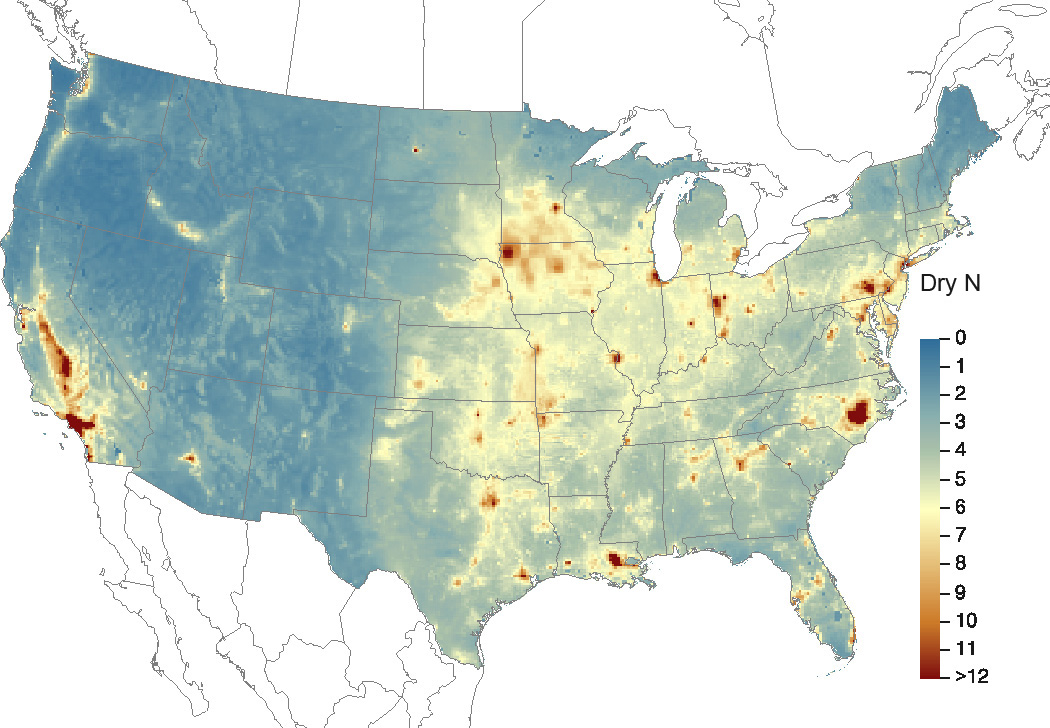 Download Figure
Source: CASTNET/CMAQ/NTN/SEARCH
Figure 9-2 TDEP Total Deposition Estimates of N (kg ha -1 yr -1) for 2015
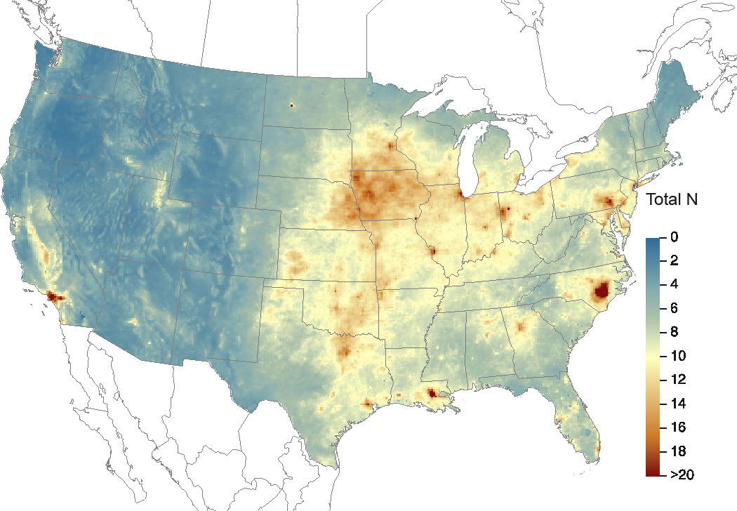 Download Figure
Source: CASTNET/CMAQ/NTN/SEARCH
Figure 9-3 TDEP Percent of Total Deposition of N from Dry Deposition for 2015
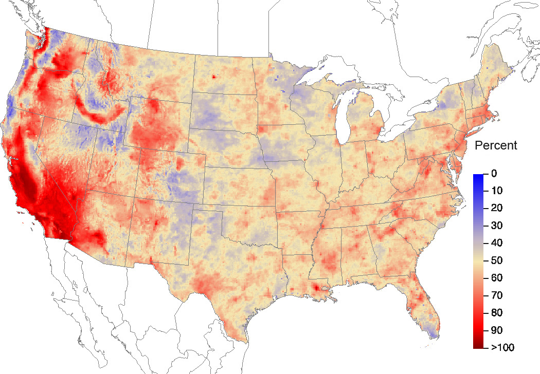 Download Figure
Source: CASTNET/CMAQ/NTN/SEARCH
Figure 9-4 TDEP Total Deposition Estimates of Reduced N Species (kg ha -1 yr -1) for 2015
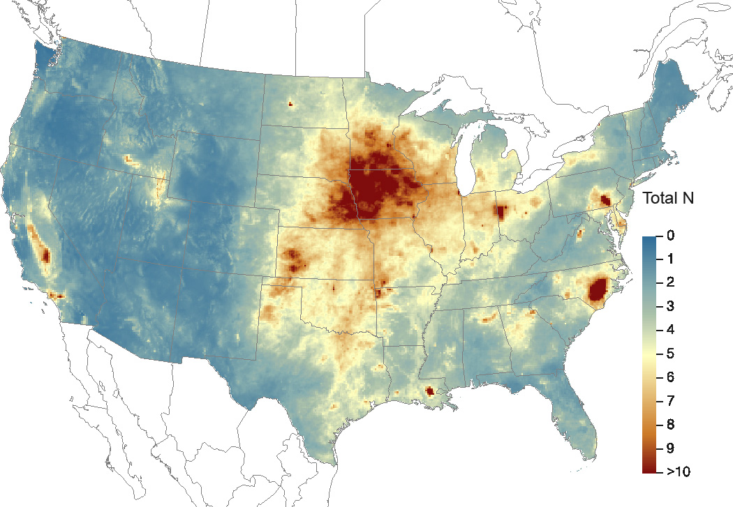 Download Figure
Source: CASTNET/CMAQ/NTN/SEARCH
Figure 9-5 TTDEP Percent of Total Deposition of Reduced N Species from Dry Deposition for 2015
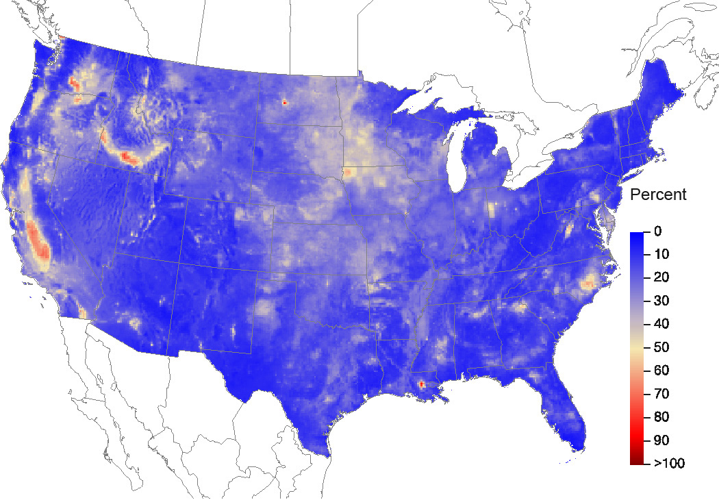 Download Figure
Source: CASTNET/CMAQ/NTN/SEARCH
Figure 9-6 TDEP Dry Deposition Estimates of Unmonitored N Species (kg ha -1 yr -1) for 2015
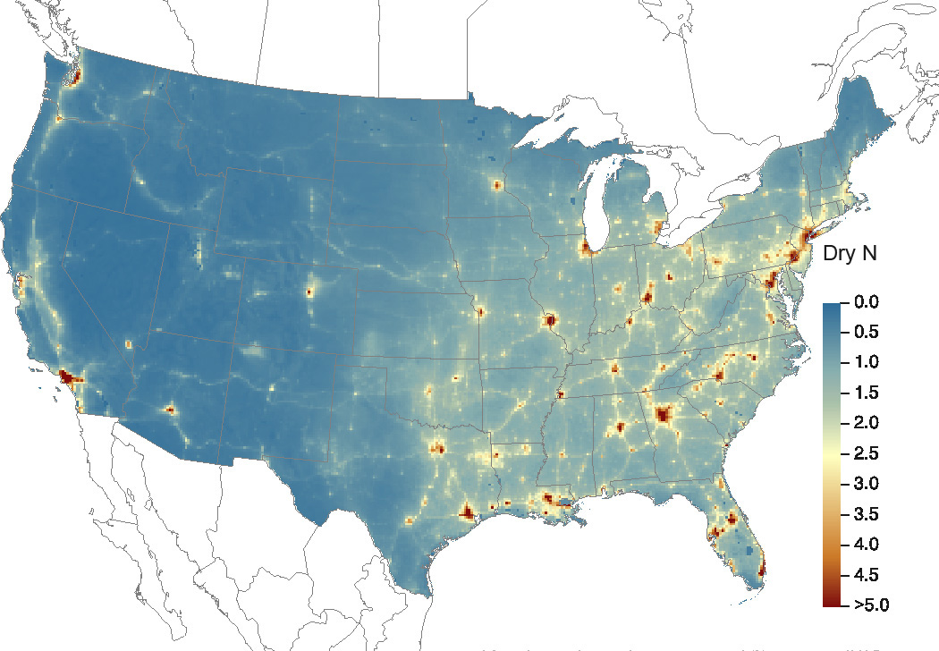 Download Figure
Source: CASTNET/CMAQ/NTN/SEARCH
Figure 9-7 TDEP Percent of Total Deposition of N from Dry Deposition of Unmonitored Species for 2015
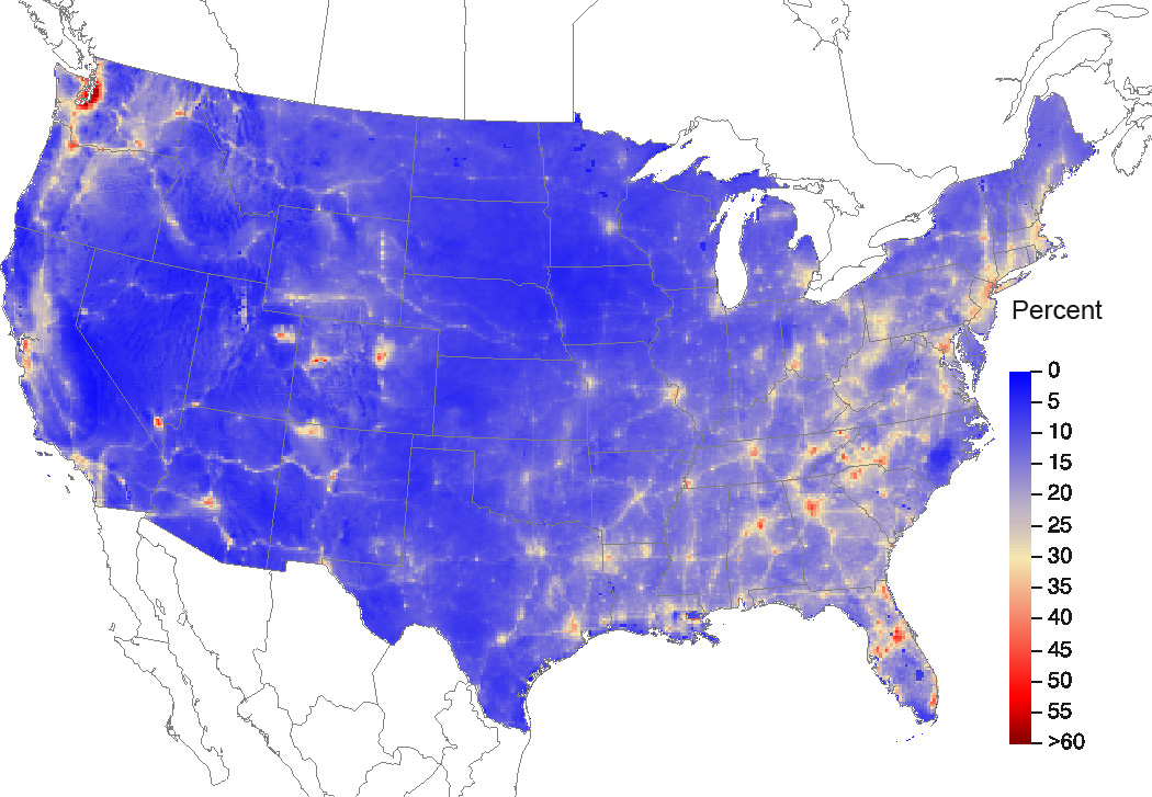 Download Figure
Source: CASTNET/CMAQ/NTN/SEARCH
Figure 9-8 TDEP Gross Dry Deposition of NH3 as N (kg ha -1 yr -1) for 2015
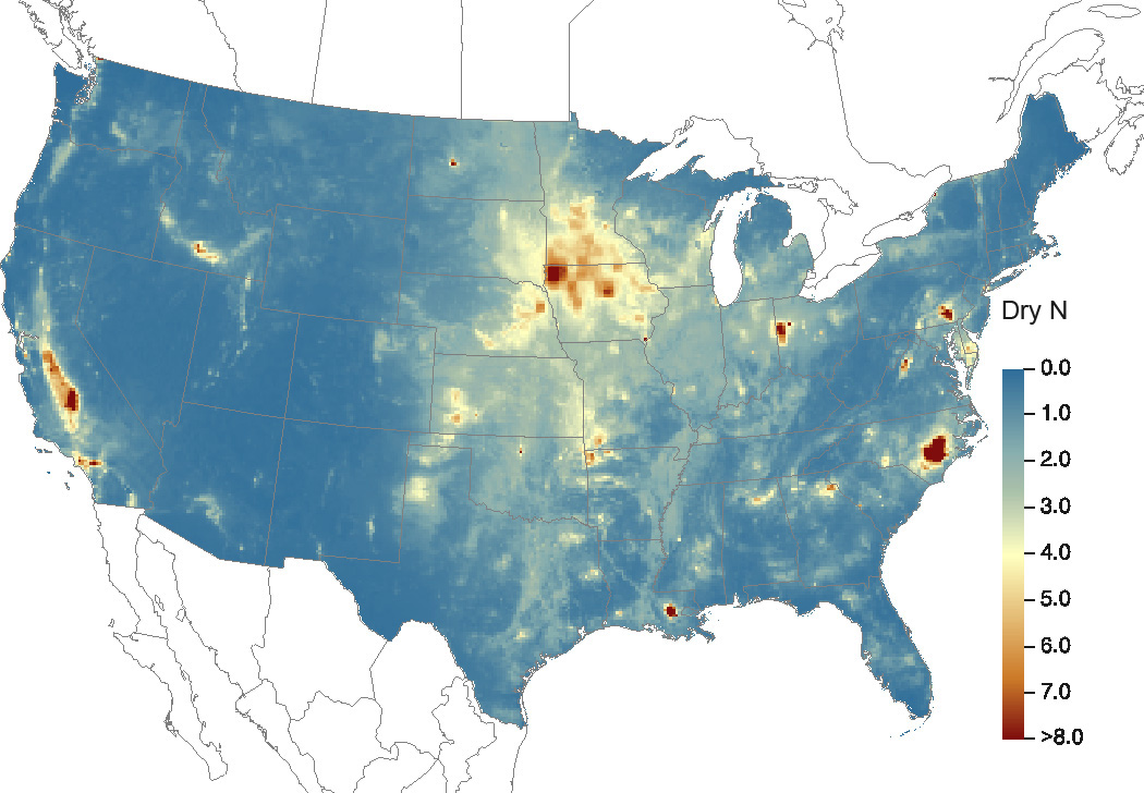 Download Figure
Source: CASTNET/CMAQ/NTN/SEARCH
Figure 9-9 TDEP Net Dry Deposition of NH3 as N (kg ha -1 yr -1) for 2015
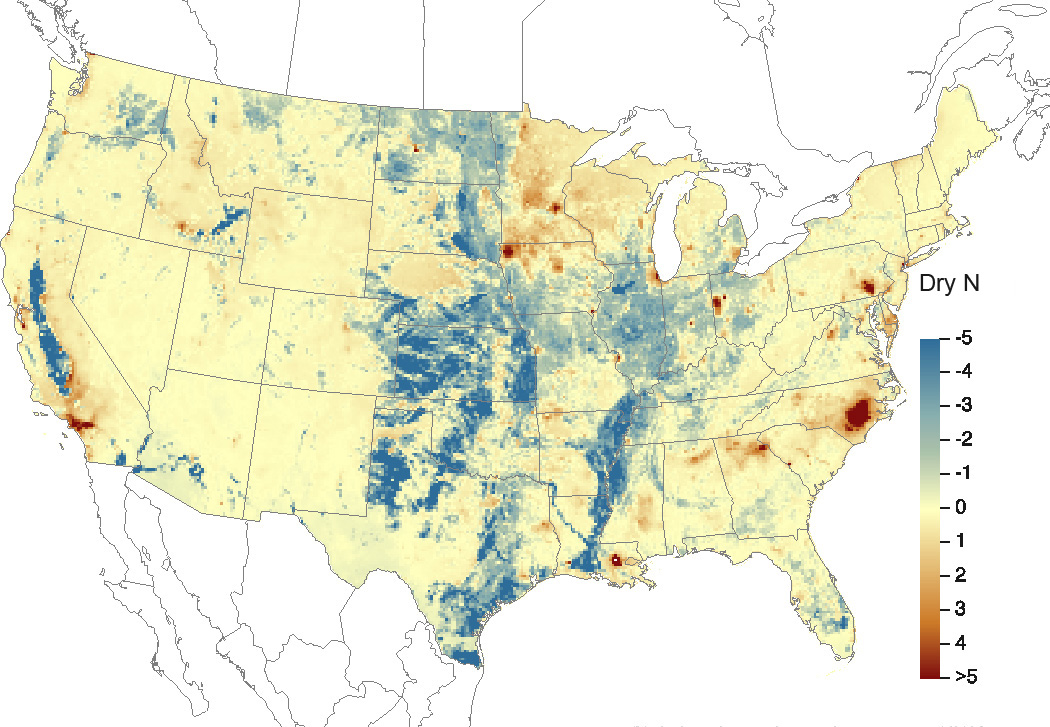 Download Figure
Source: CASTNET/CMAQ/NTN/SEARCH
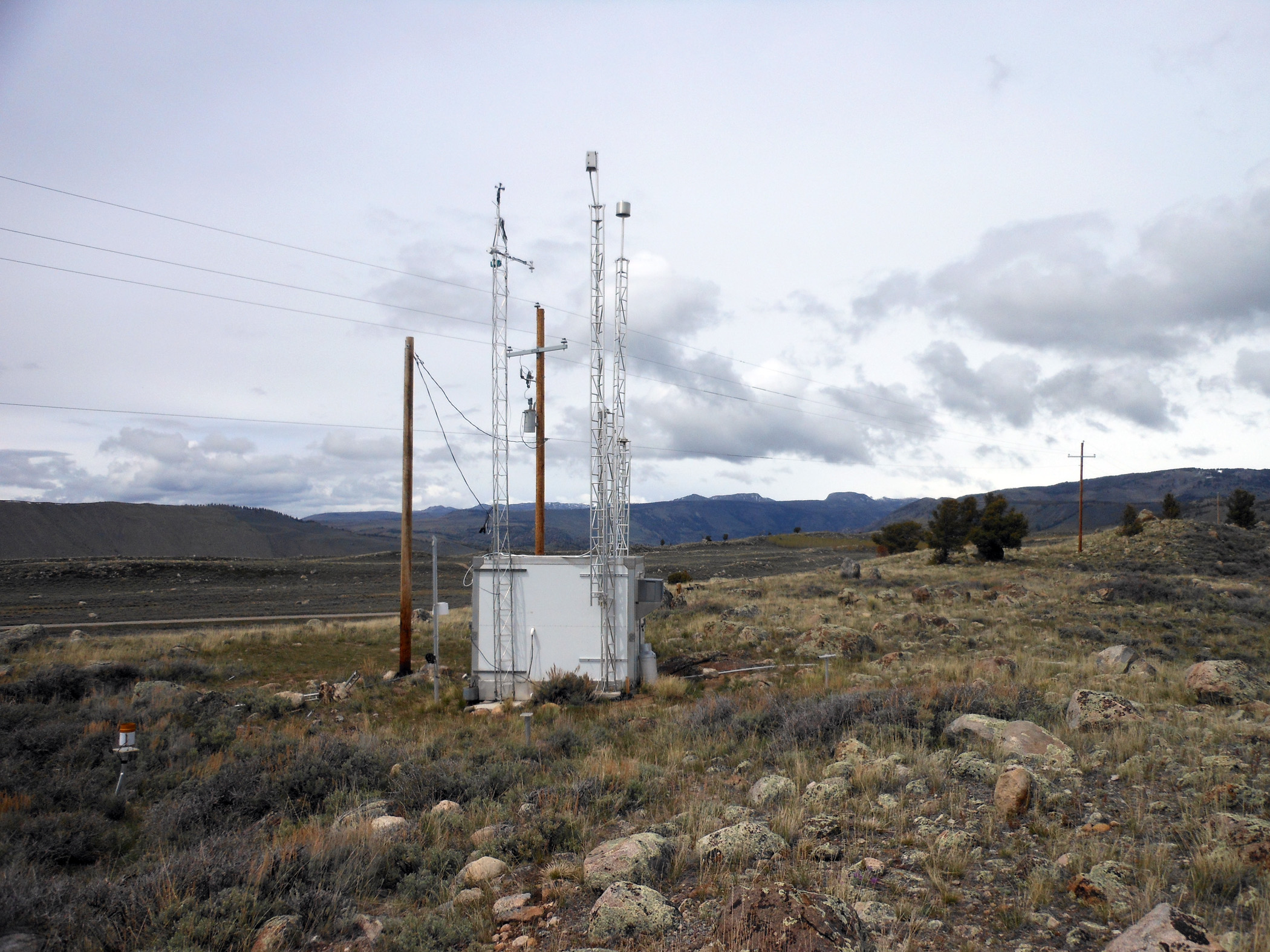
Pinedale, WY (PND165)
Chapter 10: Cloud Water, Filter Pack Pollutant, and Ammonia Concentrations at Whiteface Mountain, New York
Environmental measurements have been performed at Whiteface Mountain, NY for more than 75 years. The Atmospheric Sciences Research Center currently operates monitoring sites at the Marble Mountain Lodge and the Summit Observatory. Measurements at these two sites include seasonal cloud water, cloud water chemistry, precipitation chemistry, and filter pack concentration data. EPA operates two CASTNET small footprint, filter pack-only sites on Whiteface Mountain: a permanent site near Marble Mountain Lodge (WFM105) and a seasonal (May through October) site at the Summit Observatory (WFM007). An AMoN site was installed at Marble Mountain Lodge in late 2012. Trends in cloud water pollutant concentrations and CASTNET filter pack measurements of pollutant gases and aerosols from the Whiteface Mountain sites are presented in this chapter. Trends in ammonia concentrations from WFM105 and nearby sites are also shown.
Whiteface Mountain, located in the High Peaks region of the Adirondack Mountains, has a long history of atmospheric chemistry measurements. The Marble Mountain Lodge and the Summit Observatory are currently operated by the Atmospheric Sciences Research Center (ASRC). Marble Mountain Lodge sits on the eastern shoulder of the Whiteface Massif at an elevation of 604 m in a heavily wooded area representative of a mixed northern hardwood forest. The Summit Observatory is located on the peak of Whiteface Mountain at an elevation of 1,483 m. This location is windswept, above the tree line, and comprised primarily of bedrock with patches of thin soils. The summit microclimate is one of the coldest in the eastern United States. The short growing season and high winds limit the types of vegetation that can survive these harsh conditions (Schwab, Wolfe et al., 2016).

The first organized environmental measurements at Whiteface Mountain began in 1937 as a cooperative project between Rensselaer Polytechnic Institute, New York University, the Whiteface Mountain Highway Commission, and the Weather Bureau (now the National Weather Service) and continued until 1946. This effort provided the initial extensive meteorological data record at this location. With support from the Whiteface Mountain Authority, a wide array of meteorological instrumentation was operated throughout the late 1950s and early 1960s. The ASRC was established in 1961, and Whiteface Mountain became the main field station of the new research center. The station has been available for project work for the State University of New York schools, as well as other universities and organizations. An existing summit fire tower was replaced in 1970 with the current permanent observatory building (Figure 10-1). This structure enabled more extensive and long-term measurements at the summit. The ongoing long-term pollutant gas measurements began in 1973 when the NYSDEC started measuring O3 concentrations. Table 10-1 summarizes the timeline of the major measurement programs at the two Whiteface Mountain measurement locations (Schwab, Wolfe et al., 2016).
High volume total suspended particle (TSP) aerosol sampling at Whiteface Mountain began in 1975 and has been continuous at the Summit Observatory since 1978. The aerosol samplers collect TSP on cellulose filters and are analyzed for mass, major ions, and, as of 2007, black carbon. The NTN has operated a precipitation collection site at the Marble Mountain Lodge site since 1984. It is one of six NTN sites currently operating in the Adirondack Park. Many gas and aerosol species are incorporated into cloud water and can deposit to the environment either in precipitation or through cloud impaction, which usually occurs at elevations above 800 m. For this reason, both precipitation and cloud water samples are collected at Whiteface Mountain (Schwab, Casson et al., 2016).
| Dates* | Activity | Location | Organizations |
|---|---|---|---|
| 1937-1946 | Temperature measurements | Summit Observatory | Weather Bureau, RPI, NYU, WMHC |
| 1957 | Meteorological measurements | Summit Observatory | ASRC |
| 1963-1978 | Aerosol particle number concentration | Summit Observatory | ASRC and MML |
| 1973 | Ozone concentrations | Summit Observatory | NYSDEC |
| 1975 | High volume aerosol samples (TSP) | Summit Observatory | NYSDOH |
| 1976 | Cloud collection (seasonal) | Summit Observatory | ASRC/EPA/ALSC |
| 1976 | Precipitation collection | MML | ASRC/NYSDEC/NADP |
| 1984 | Ozone and other pollutant gases | MML | NYSDEC/ASRC |
| 1988 | Pollutant and ozone precursor gases | Summit Observatory | ASRC |
| 1999 | PM2.5 mass concentration (filter samples and continuous) | MML | NYSDEC |
| 2001 | PM2.5 chemical speciation (filter samples) | MML | EPA/CSN |
| 1987-1993 2012 | Filter pack measurements | MML | EPA/CASTNET |
| 2012 | AMoN NH3 | Summit Observatory | NADP |
| 2015 | Filter pack measurements | Summit Observatory | EPA/CASTNET |
Note: *When no end date is given, the specified activity is continuing.
Abbreviations used in Table 10-1:
- ALSC – Adirondack Lake Survey Corporation
- ASRC – Atmospheric Sciences Research Center, University at Albany, State University of New York
- CSN – Chemical Speciation Network
- MML – Marble Mountain Lodge
- NADP – National Atmospheric Deposition Program
- NYSDEC – New York State Department of Environmental Conservation
- NYSDOH – New York State Department of Health
- NYU – New York University
- WMHC – Whiteface Mountain Highway Commission
Source: Schwab, Wolfe et al. (2016)
Cloud Water Measurements
Cloud water collection at the station started in 1976 when the ASRC began a routine program of continuous cloud water collection and pH analysis (Schwab, Wolfe et al., 2016). These efforts later became a part of the Mountain Cloud Chemistry Project (MCCP), which operated from 1986 to 1989 and was administered by the Forest Response Program of the National Acid Precipitation and Assessment Program (NAPAP) and was sponsored by the EPA. MCCP data were used in the NAPAP Integrated Assessment to evaluate the role of airborne chemicals in the changing condition of forests (National Science and Technology Council, 2005).
The MCCP was followed several years later by the Mountain Acid Deposition Program (MADPro), which officially operated under CASTNET from 1993 through 2011 during the warm seasons. MADPro’s two main objectives were to develop cloud water measurement systems geared towards operating in a network setting and update the Appalachian Mountains cloud water concentrations and deposition data collected by NAPAP during MCCP. MADPro consisted of three main sampling stations: Whiteface Mountain, NY; Whitetop Mountain, which was located in the Mount Rogers National Recreation Area in Virginia; and Clingmans Dome, which was located in the Great Smoky Mountains National Park in Tennessee. Of these three sites, Whiteface Mountain is the only site still in operation today. Whitetop Mountain closed after the 1999 season, and the Clingmans Dome site closed after the 2011 season. After the 2000 season, Whiteface Mountain cloud water collection activities have been sponsored by the NYSDEC and the New York State Energy Research and Development Authority, and the site, WFM300, is operated by the Adirondack Lake Survey Corporation. The particle volume monitor, which is used to determine the presence of a cloud as well as the liquid water content of the cloud, is shown in Figure 10-2. The cloud water collector is shown in Figure 10-3. Figure 10-4 shows concentrations in microequivalents per liter (μeq/L) of the major ions, SO4-, NO3-, and NH4+ , in cloud water from 2001 through 2015. SO42-, NO3- , and NH4+ all show downward trends.
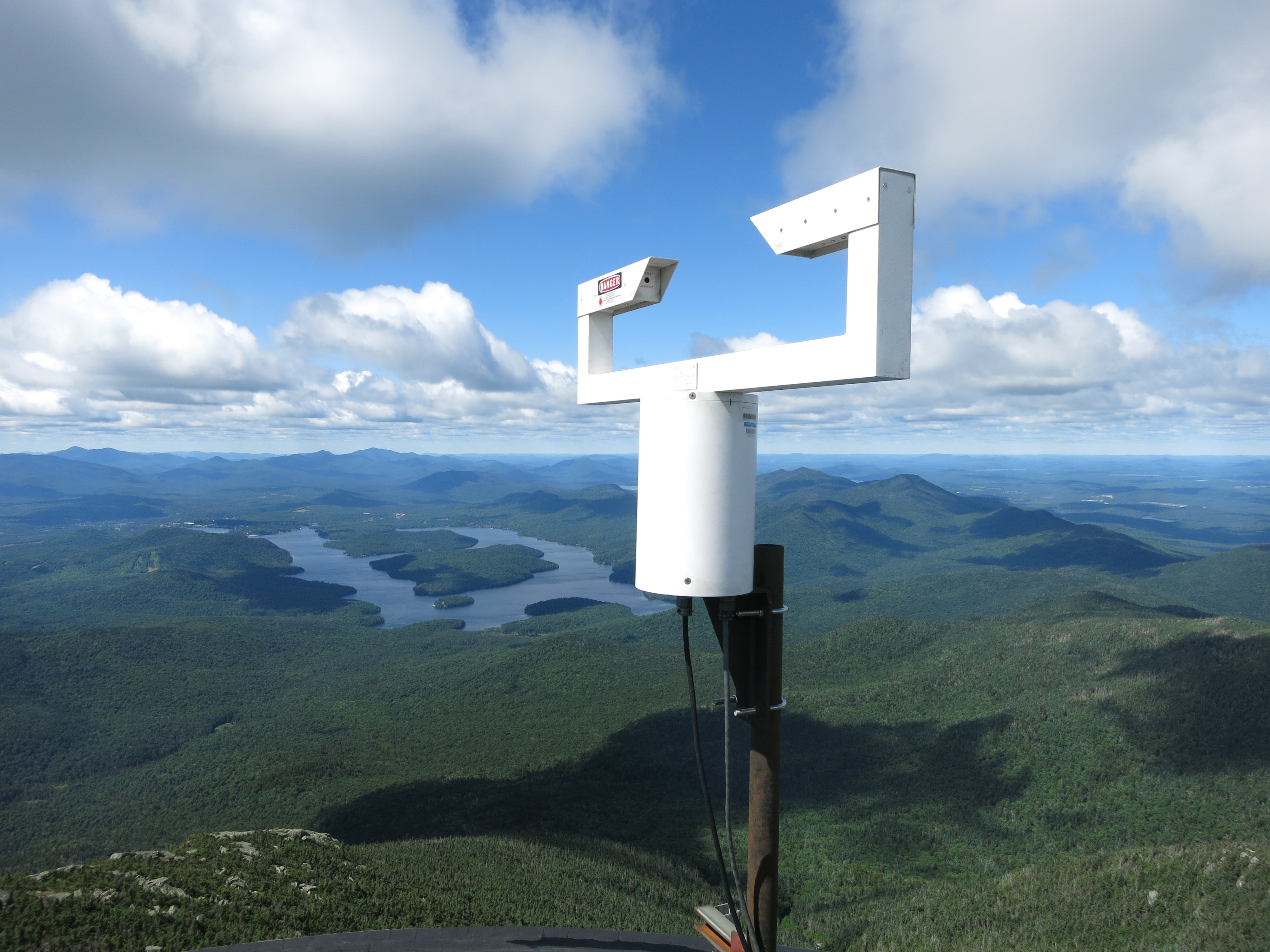
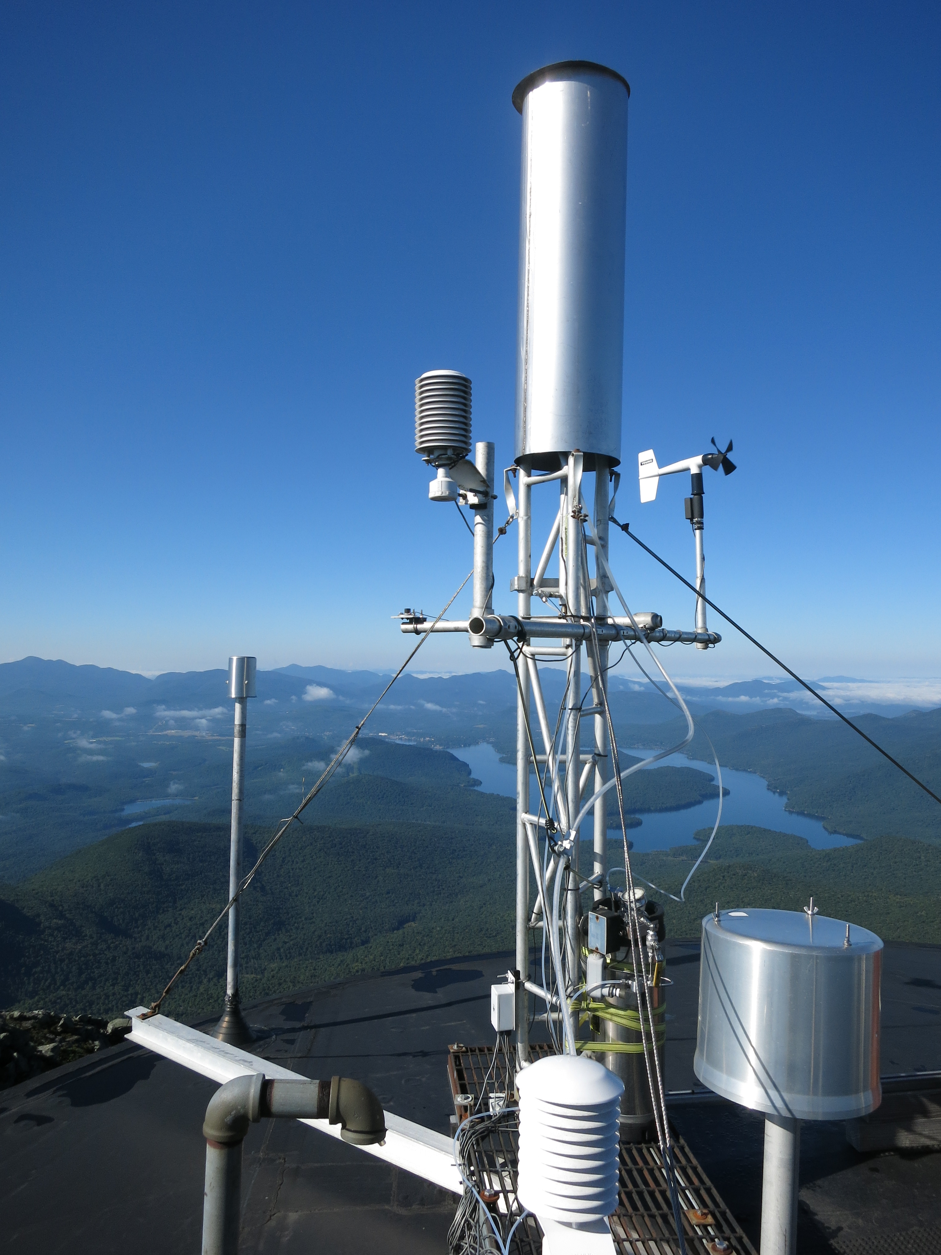
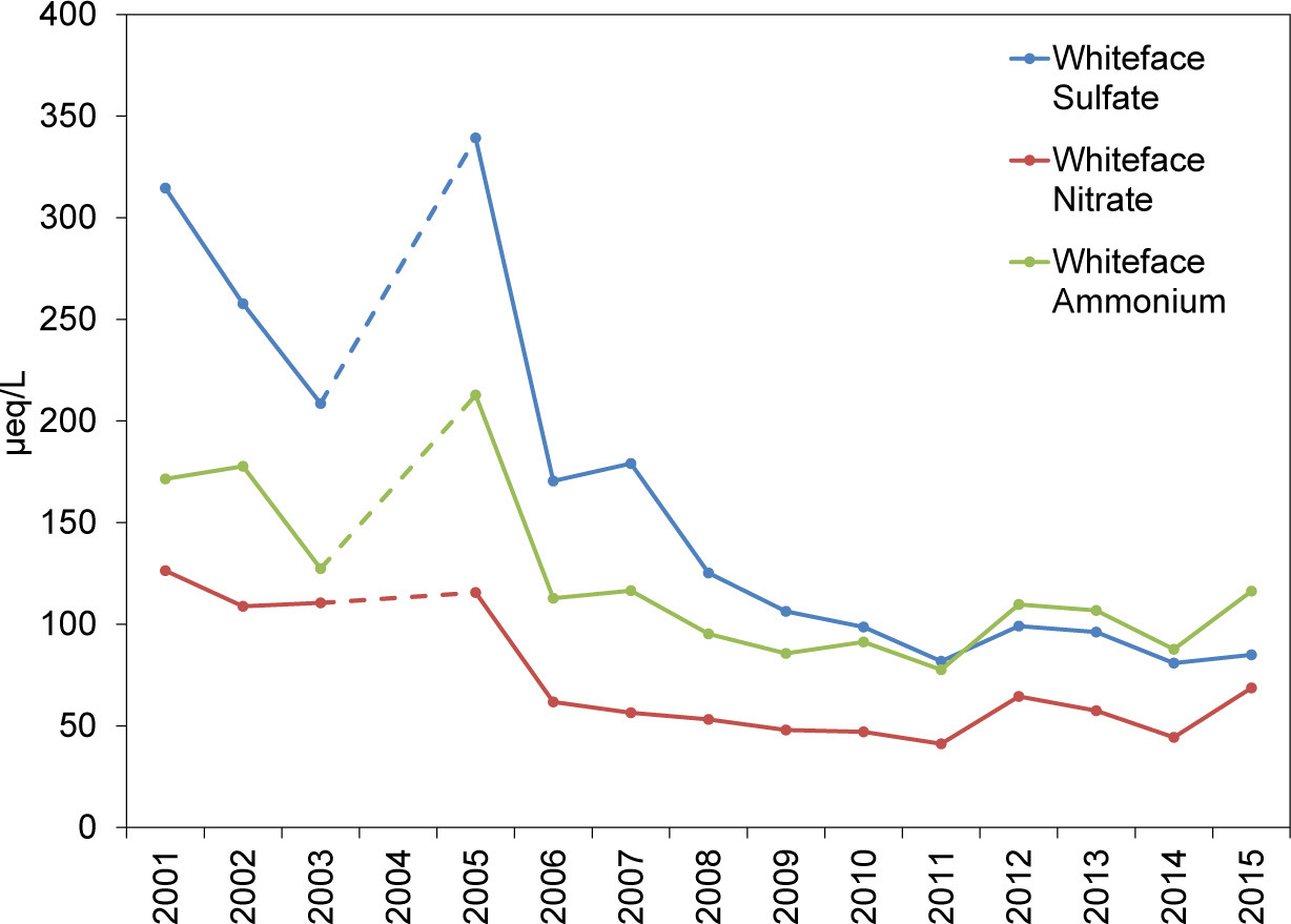
Filter Pack Measurements
A CASTNET small footprint filter pack site (WFM105) was installed near the NTN precipitation collector at Marble Mountain Lodge in 2012 (Figure 10-5). Dry deposition data estimated from filter pack concentrations and wet deposition data calculated from the precipitation concentrations allow for estimation of total deposition at this location. A CASTNET filter pack (WFM007) was also installed at the Summit Observatory in 2015 (Figure 10-6). Total deposition values can now be estimated for the summit location as well, albeit with NTN precipitation data from the Marble Mountain Lodge site. Ideally, data from an NTN collector at the summit would be preferable. Precipitation collection at the summit would enable direct comparison of total deposition between the two locations. Even without the NTN collector at the summit site, comparison of dry deposition values between the two CASTNET filter pack sites is still useful for discerning the contribution from cloud water to total deposition.
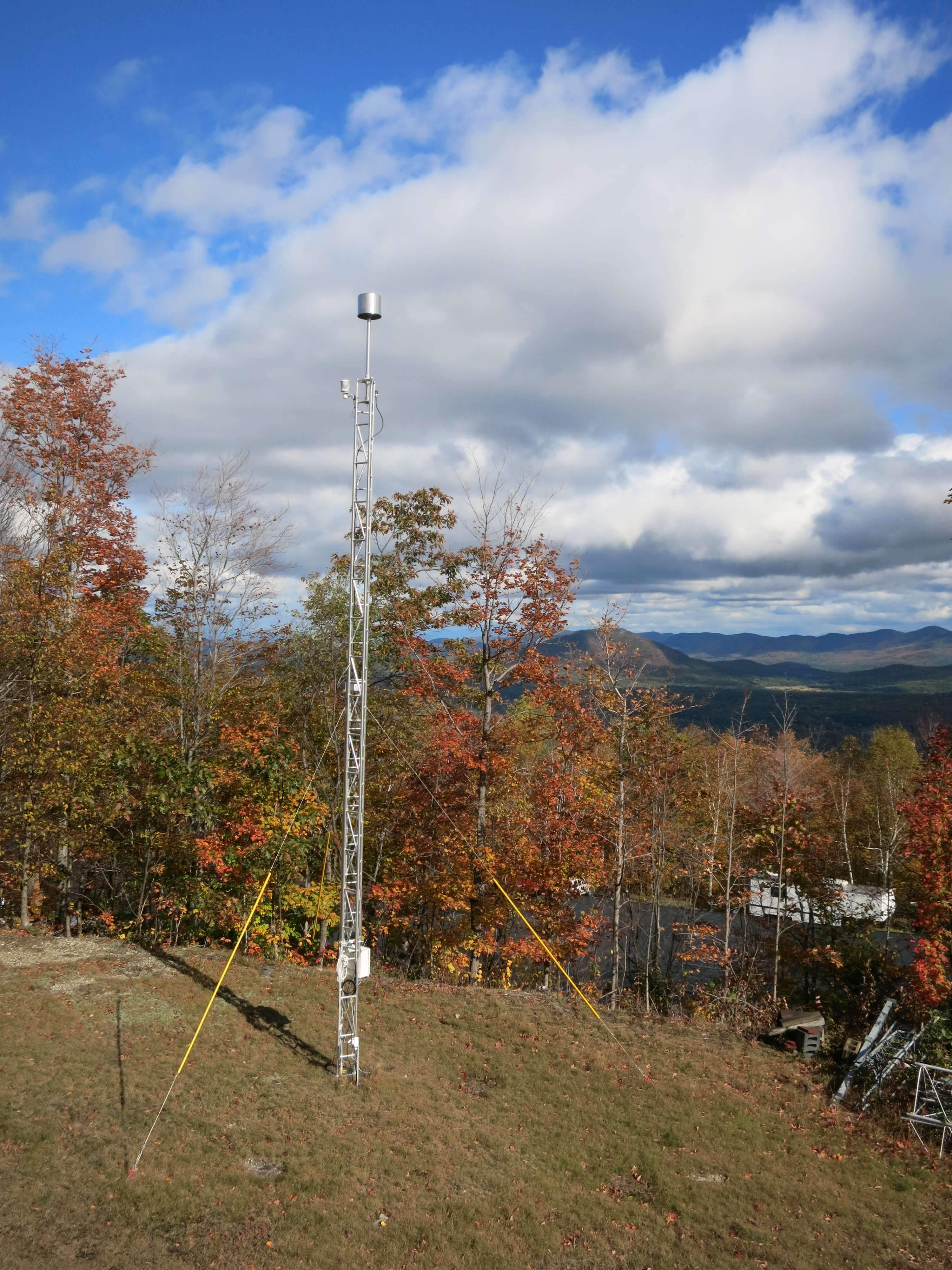
Figures 10-6 CASTNET Filter Pack (WFM007) at the Summit Observatory
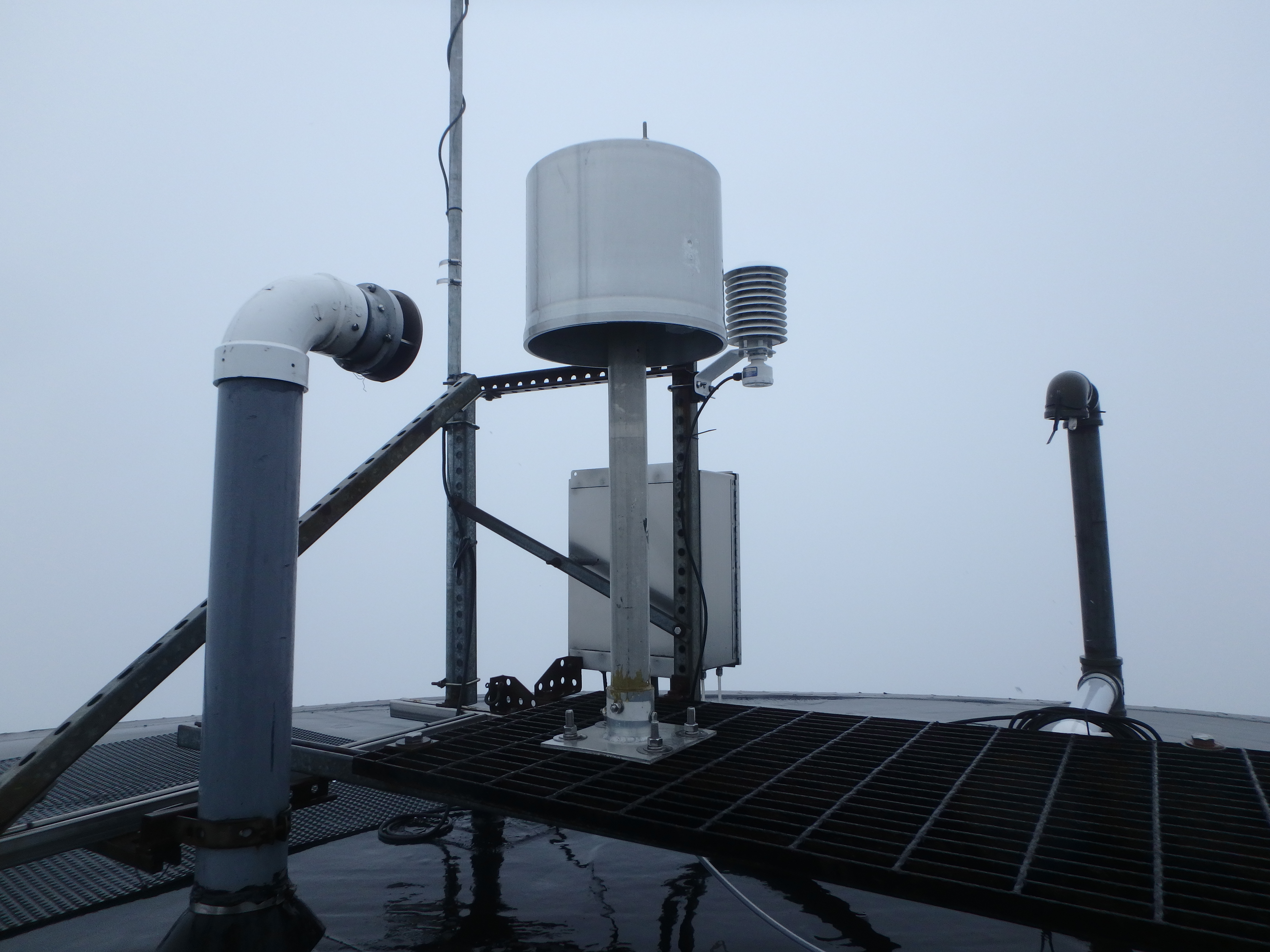
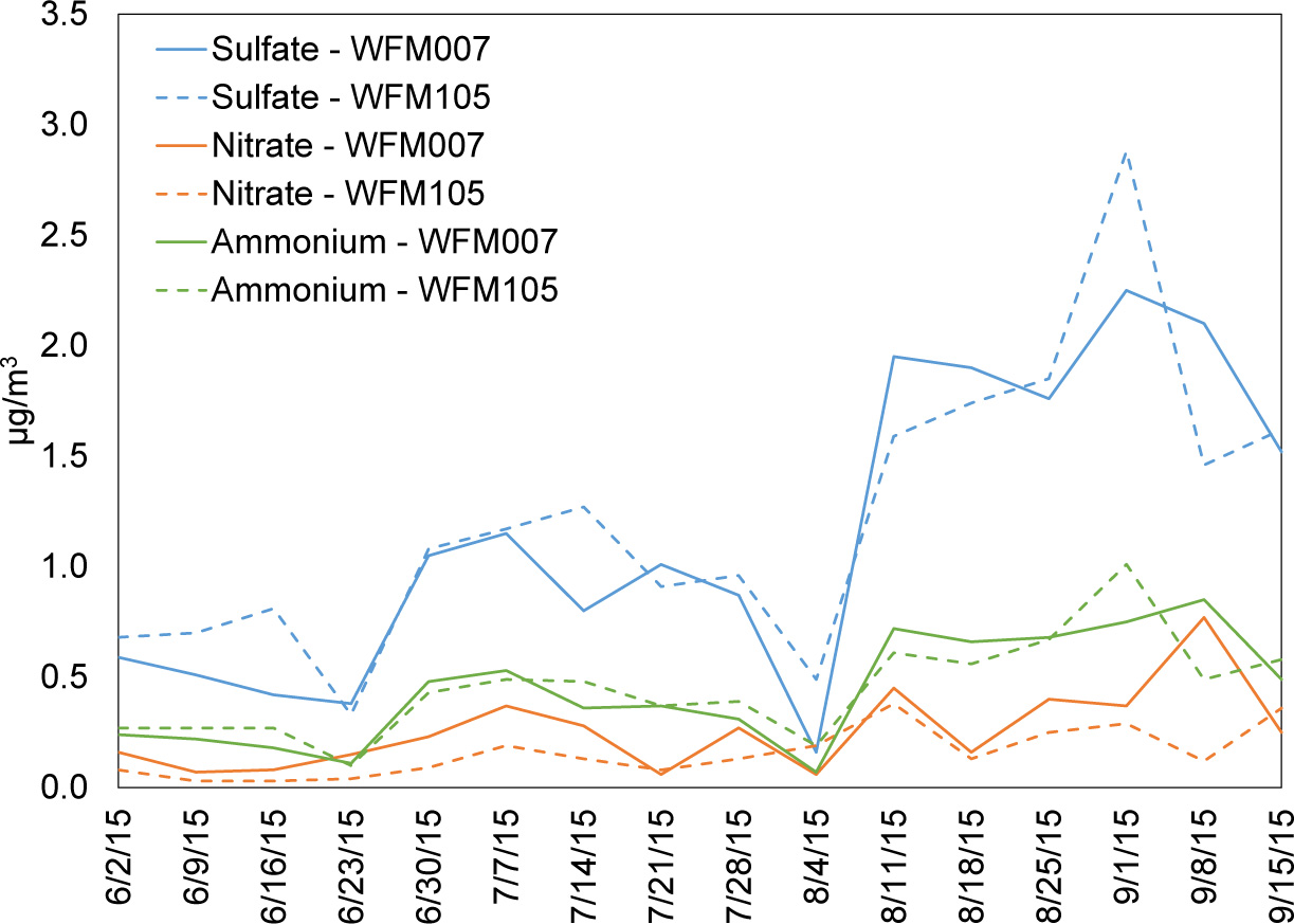
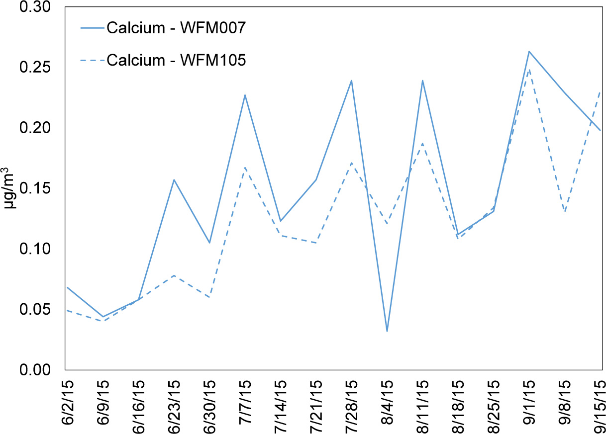
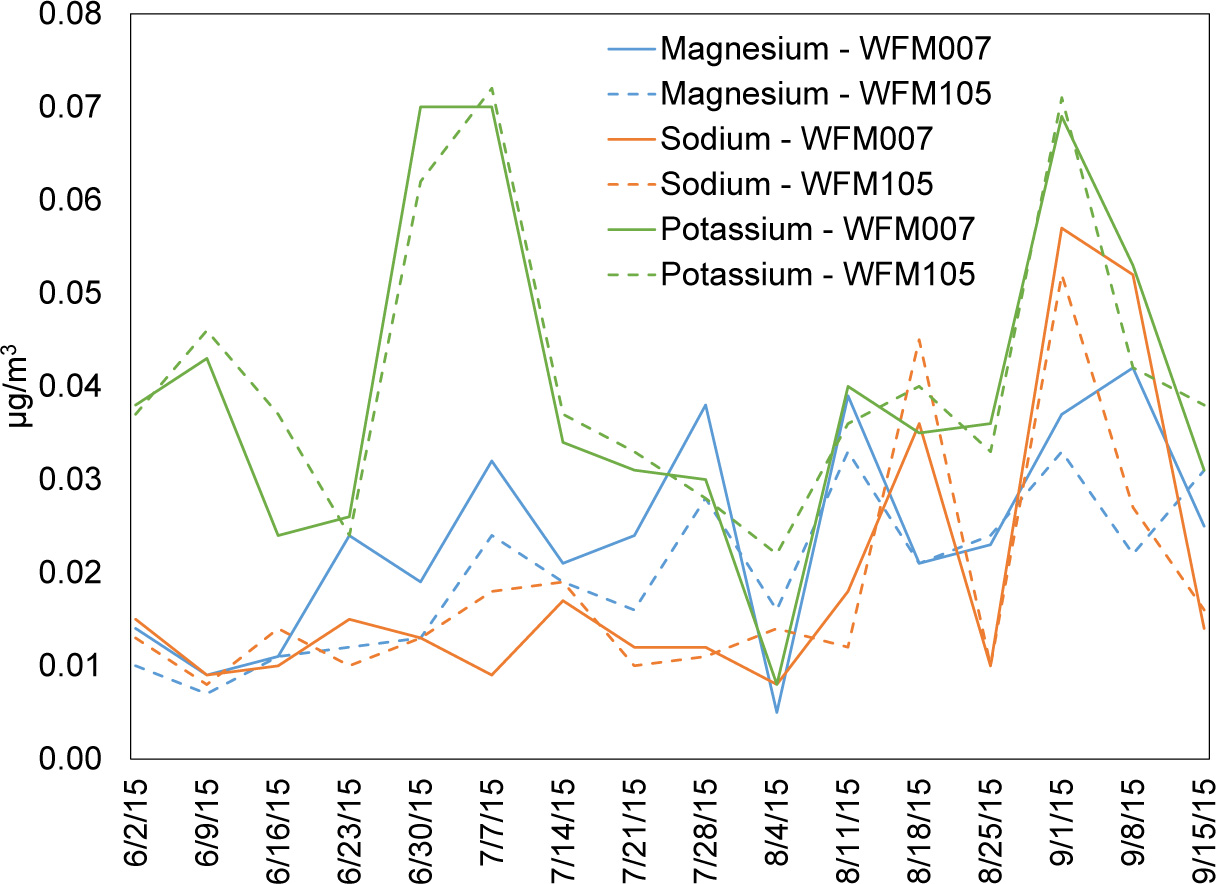
Including the two sites at Whiteface Mountain, six CASTNET filter pack systems were operated in New York along with one filter pack in Vermont and one in New Hampshire (Figure 1-1 and Appendix A). Figures 10-10, 10-11, and 10-12 present time series of weekly NH + , SO2-, and total NO- 443 concentrations measured during the summer of 2015 at the eight sites. Lower concentrations were measured at the more remote sites and higher concentrations at the downstate sites at CTH110, NY and CAT175, NY.
Ammonia Measurements
AMoN began monitoring biweekly NH3 gas concentrations using passive samplers in 2007 (Chapter 5). An AMoN station was installed at the Marble Mountain Lodge site in late 2012. Currently, there are nine AMoN sites in upstate New York and one site each in Vermont and New Hampshire. Figure 10-13 shows biweekly NH3 concentrations for five New York sites, one Vermont site, and one New Hampshire site. Trend lines were plotted for the Marble Mountain Lodge (NY98) and Ithaca, NY (NY67/CTH110) sites to illustrate a slight increase in NH3 concentrations since November 2012. Figure 10-14 shows time series of 2-week NH3 concentrations measured at NY67/CTH110 and the Cary Institute (NY16) from October 2007 through February 2016. Linear regression suggest slight increases in NH3 concentrations.
Figure 10-15 compares AMoN ambient NH3 concentrations (μg/m 3 ) and NTN precipitation NH4+ concentrations [milligrams per liter (mg/L)] measured at Marble Mountain Lodge over three years. Ambient NH3 concentrations were not correlated with NH4+ concentrations in precipitation.
Figure 10-10 Time Series of Weekly Filter Pack NH4+ Concentrations measured at Eight CASTNET Sites
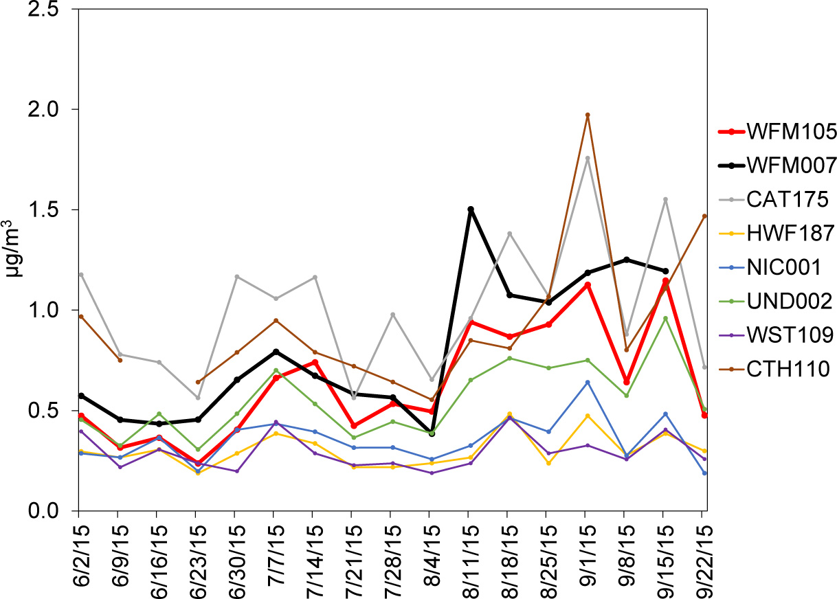 Download Figure
Figure 10-11 Time Series of Weekly Filter Pack SO42- Concentrations measured at Eight CASTNET Sites
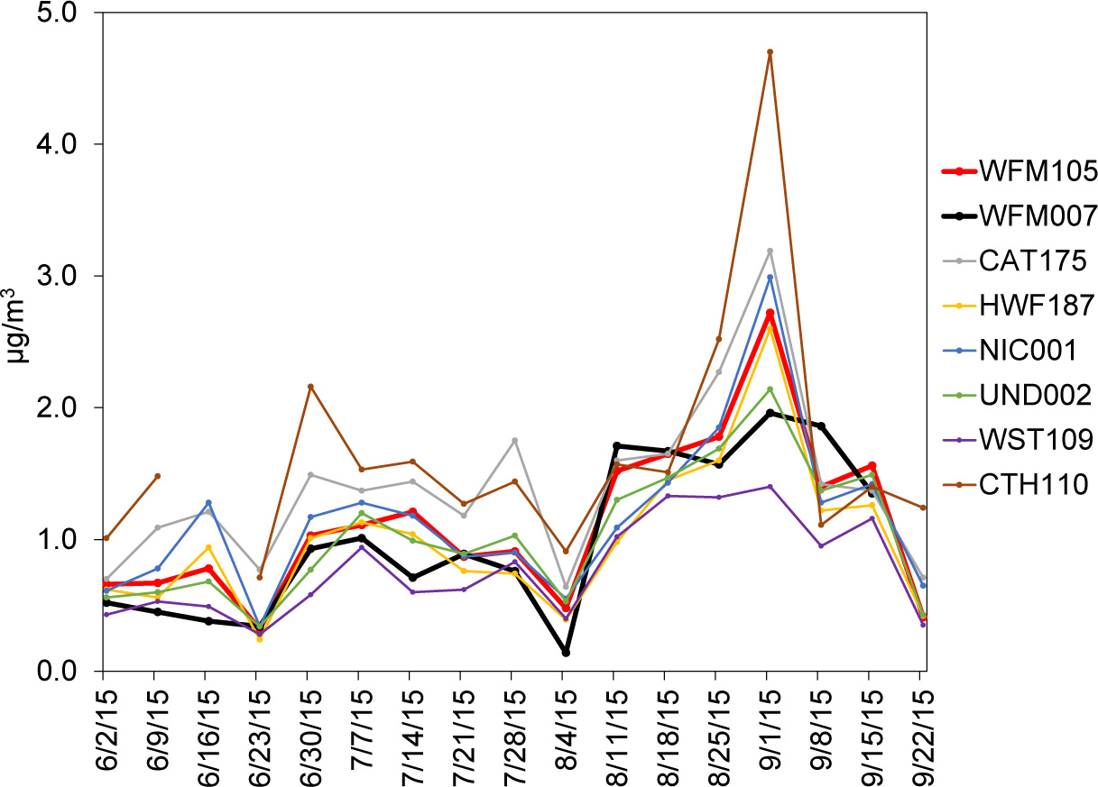 Download Figure
Figure 10-12 Time Series of Weekly Filter Pack NO3- Concentrations measured at Eight CASTNET Sites
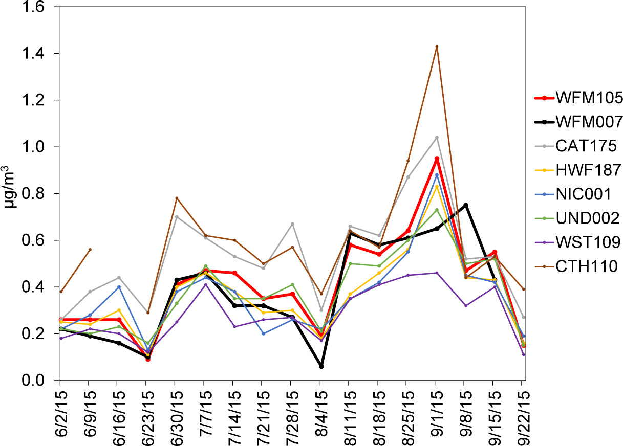 Download Figure
Figure 10-13 Time Series of Biweekly NH3- Concentrations measured at Seven AMoN Sites
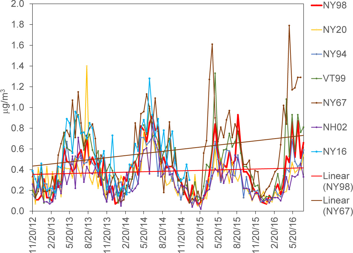 Download Figure
Figure 10-14 Time Series of Biweekly NH3- Concentrations at AMoN Sites NY67 and NY16
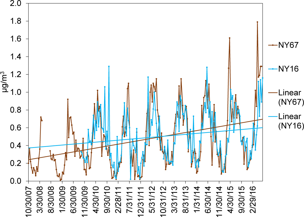 Download Figure
Figure 10-15 Comparison of AMoN Ambient NH3 Concentrations (left axis) and NTN Precipitation NH4+ Concentrations (rightaxis) at Marble Mountain Lodge
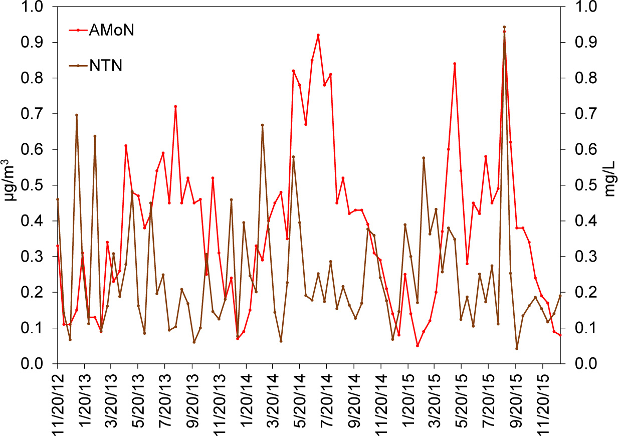 Download Figure
Chapter 11: Trends in Atmospheric Deposition
CASTNET was designed to provide estimates of the dry deposition of nitrogen and sulfur pollutants, base cations, and chloride across the United States. EPA used the NADP Total Deposition Hybrid Method to assess the status of dry and wet deposition for 2015. Total deposition was calculated as the sum of estimated dry and wet deposition.
Gaseous and particulate sulfur pollutants, base cations, and chloride are deposited to the environment through dry and wet atmospheric processes. A principal goal of CASTNET is to estimate the rate of dry deposition of these compounds from the atmosphere to sensitive ecosystems. The NADP TDEP Hybrid Method (EPA, 2015c; Schwede and Lear, 2014) was used to estimate dry and wet deposition. Dry and wet deposition rates were summed to obtain total deposition across the United States.
Sulfur Deposition
Figure 11-1 shows a map of TDEP dry deposition rates of sulfur (S) for 2015. Estimated rates of total deposition of sulfur for 2015 are given in Figure 11-2. The magnitude of the deposition fluxes is illustrated by the shading in the figure legends. The percentage of total deposition of S due to dry deposition is shown in Figure 11-3.
Deposition of Base Cations and Chloride
A map of 2015 estimated total deposition of base cations (Ca 2+, K + , Mg 2+, and Na + ) is given in Figure 11-4. Figure 11-5 provides estimated rates for 2015 for total deposition of Cl -.
Sand Mountain, AL (SND152)
Figure 11-1 TDEP Dry Deposition Estimates of S (kg ha -1 yr -1) for 2015
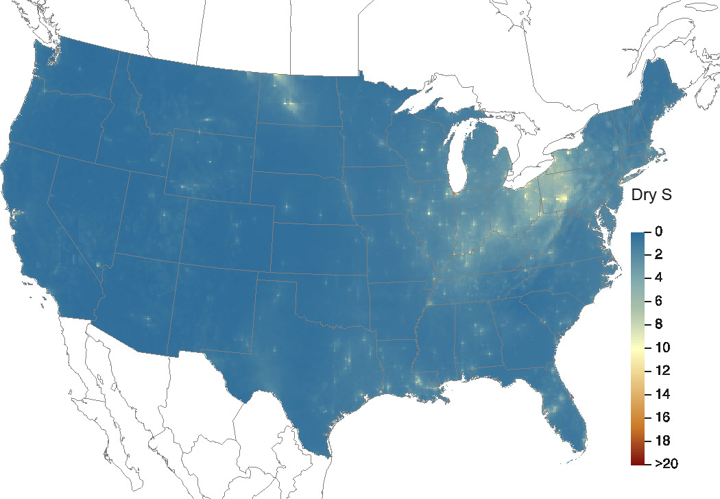 Download Figure
Source: CASTNET/CMAQ/NTN/SEARCH
Figure 11-2 TDEP Total Deposition Estimates of S (kg ha -1 yr -1) for 2015
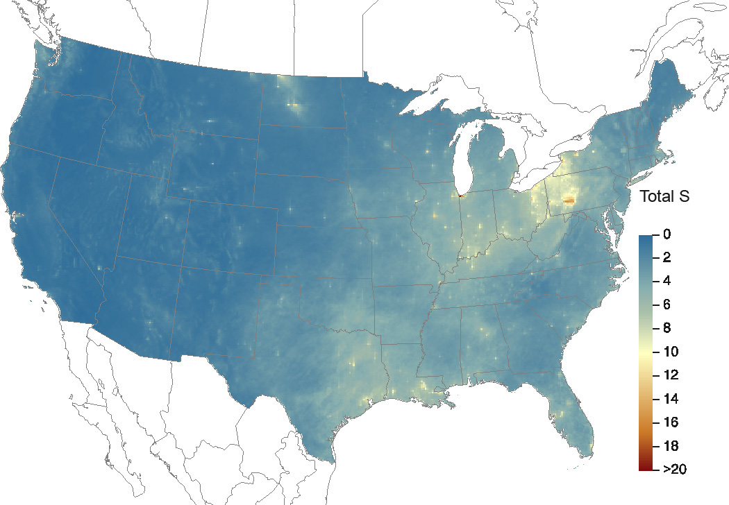 Download Figure
Source: CASTNET/CMAQ/NTN/SEARCH
Figure 11-3 TDEP Percent of Total Deposition of S from Dry Deposition for 2015
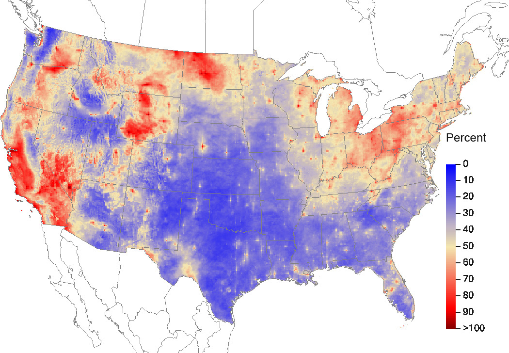 Download Figure
Source: CASTNET/CMAQ/NTN/SEARCH
Figure 11-4 TDEP Total Deposition Estimates of the Base Cations Ca 2+, K + , Mg 2+, Na + (kiloequivalents per hectare per year) for 2015
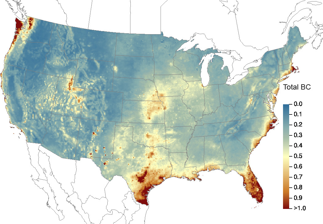 Download Figure
Source: CASTNET/CMAQ/NTN/SEARCH
Figure 11-5 TDEP Total Deposition Estimates of Total Cl - (kg ha -1 yr -1) for 2015
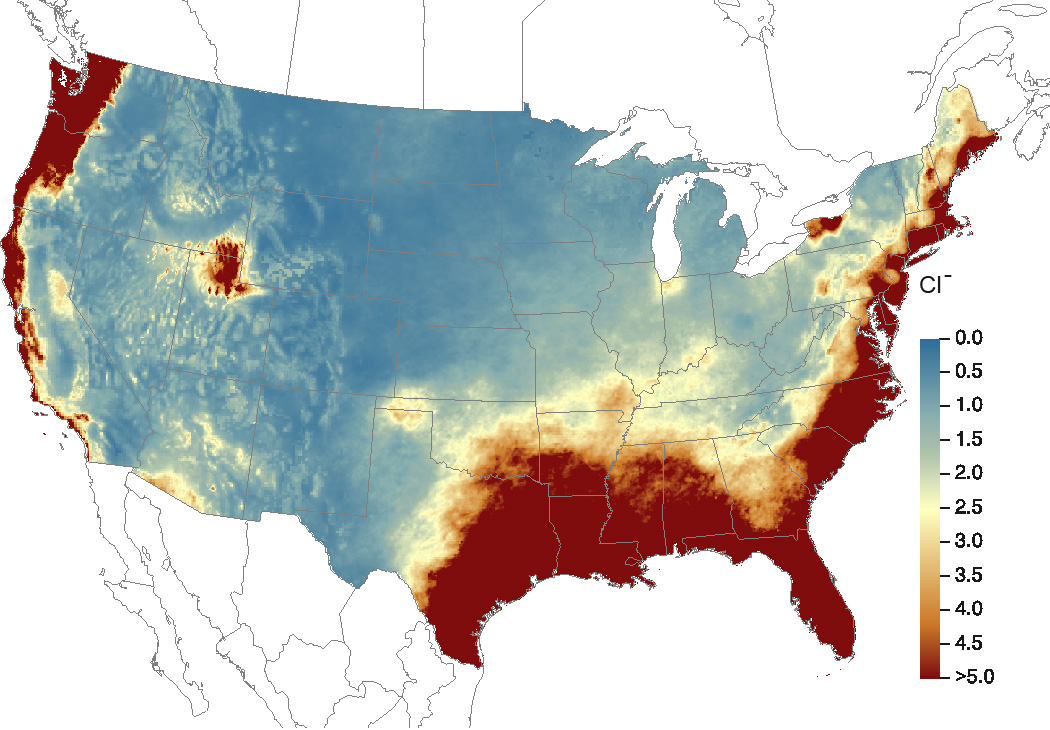 Download Figure
Source: CASTNET/CMAQ/NTN/SEARCH
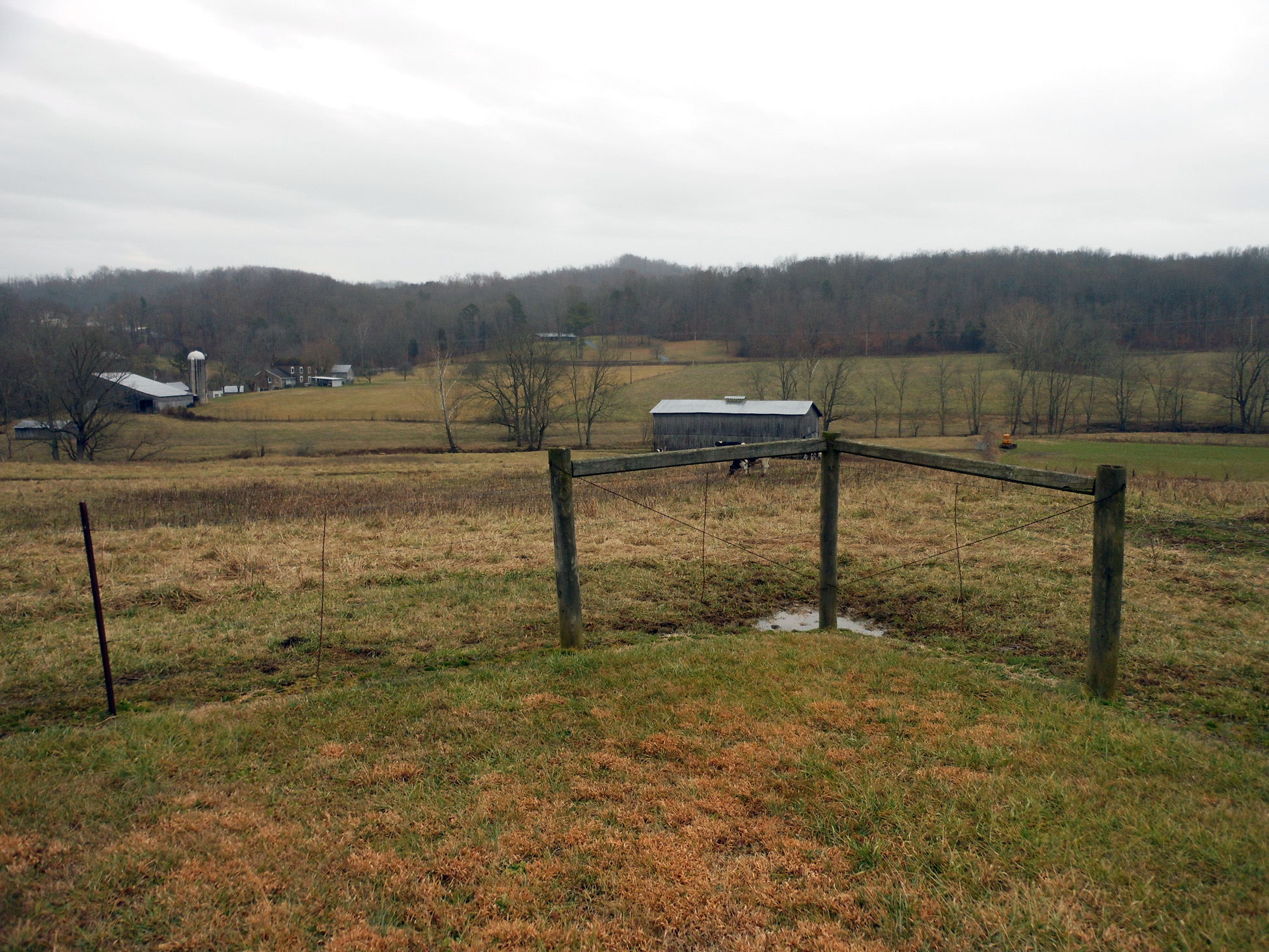
Speedwell, TN (SPD111)
Chapter 12: Improved Forest Health in the Eastern United States
Reduced power plant and industrial combustion emissions implemented under the Clean Air Act have resulted in improved air quality and health of forest ecosystems over the last 30 years. CASTNET data and data from other monitoring programs, which are archived and documented in the EPA AQS, were used to assess the extent to which ambient concentrations of ozone and total nitrate have declined and to understand the corresponding changes in forest ecosystem health. Ambient ozone can enter a plant through stomatal pores in leaves and cause significant cellular damage that may compromise the plant’s photosynthetic capacity leading to reduced growth and/or reproduction of plants. Ozone stress also increases the susceptibility of plants to disease, insects, fungus, and other environmental stresses (e.g., harsh weather). Ozone is formed primarily from photochemical reactions between volatile organic compounds and nitrogen oxides. Thus, reducing nitrogen oxides emissions would in turn lower ground-level ozone concentrations and help to improve forest ecosystem health. This chapter discusses how nitrogen oxides emission reduction programs have resulted in improved air quality, decreased ozone levels, and improved forest health.
Methods
Ground-level O3 has been shown in numerous studies to have a strong effect on the health of many plants, including a variety of commercial and ecologically important forest tree species throughout the United States. (Ollinger et al., 1997; EPA, 2007). Assessing the impact of ground-level O3 on forests in the eastern United States involved analyzing the risk to tree species from ambient O3 concentrations and accounting for the prevalence of those species within a forest. As a way to quantify the risk to particular trees, concentration-response (C-R) functions, which relate O3 exposure to tree response, were calculated (EPA, 2014b). Tree seedling C-R functions were determined by exposing tree seedlings to different O3 levels and measuring reductions in growth as “biomass loss.” In areas where certain species dominate the forest community, the biomass loss from O3 can be significant. In this analysis, biomass loss was used as an indicator for the effects of O3 on the forest ecosystem.
Common tree species in the eastern United States that are sensitive to O3 include black cherry (Prunus serotina), yellow poplar (Liriodendron tulipifera), sugar maple (Acer saccharum), eastern white pine (Pinus strobus), Virginia pine (Pinus virginiana), red maple (Acer rubrum), and quaking aspen (Populus trenuloides; Chappelka and Samuelson, 1998). To estimate the biomass loss for forest ecosystems across the eastern United States, the biomass loss for each of the seven tree species was calculated using the 3-month, 12-hour W126 exposure metric at each monitoring site, along with each tree’s individual C-R functions. The W126 exposure metric is a biologically based, cumulative exposure index that places a greater weight on the higher hourly O3 concentrations (Heck and Cowling, 1997). The W126 exposure metric was calculated using O3 data from the rural CASTNET and urban AQS networks and averaged over a 3-year period to mitigate the effect of variations in meteorological and soil moisture conditions. The biomass loss estimate for each species was then multiplied by its prevalence in the forest community using the U.S. Department of Agriculture’s Forest Service IV index of tree abundance calculated from Forest Inventory and Analysis measurements (Prasad and Iverson, 2003). This analysis compared two time periods, 2000–2002 (e.g., beginning of NOx Budget Trading Program) and 2012–2014 (most recent modeling years) and demonstrates the benefit of decreasing O3 concentrations to forest ecosystems.
Results
Ambient Total Nitrate and Ozone Concentrations
Based on eastern reference site data from 1989 through 2014, the annual mean total NO3- concentration declined 45 percent from 3.1 ppb to 1.7 ppb in the eastern United States. (Figure 12-1 and Chapter 4). Rural DM8A O3 concentrations decreased from 85 ppb to 66 ppb (22 percent) from 2000–2002 to 2012–2014 in the eastern United States (Figure 12-2 and Figure 2-3 in Chapter 2).
Figure 12-1 Annual Mean Total NO3- Concentrations, 1989–1991 versus 2012–2014
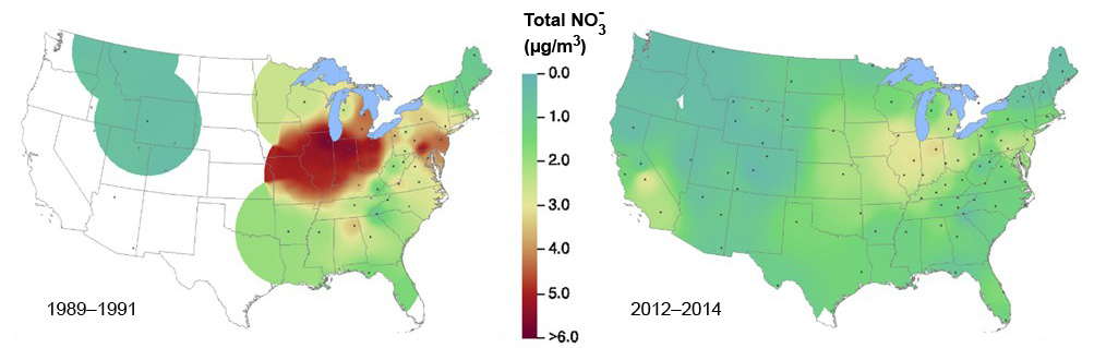 Download Figure
Source: https://www3.epa.gov/castnet/maps/airconc.html
Figure 12-2 Three-year Average of Fourth Highest DM8A O3 Concentrations, 2000–2002 versus 2012–2014
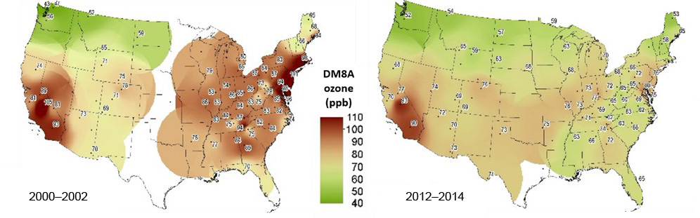 Download Figure
Source: https://www3.epa.gov/castnet/maps/airconc.html
Effects of Decreased Ozone Pollution on Forest Biomass
Forest areas with significant biomass loss (EPA, 2007) 1 because of O3 exposure decreased from 33 percent to 5 percent from 2000–2002 to 2012–2014 (Figure 12-3) for all seven tree species that were modeled across their ranges in the eastern United States. Of these, black cherry and yellow poplar are the most sensitive to O3. Comparing data from 2000–2002 versus 2012–2014, total land area in the region with significant biomass loss decreased from 15.3 to 5.1 percent for black cherry and from 3.1 to 0.0 percent for yellow poplar. Significant biomass loss for the remaining five species (red maple, sugar maple, quaking aspen, Virginia pine, and eastern white pine) is zero. This is in contrast to the period 2000–2002, when 34 percent of range loss could be attributed to O3 exposure. While this modeled improvement in forest health cannot be exclusively attributed to Clean Air Act-produced NOx emission reduction programs, e.g., NOx Budget Trading Program and Clean Air Interstate Rule, it is likely that NOx emission reduction programs and the corresponding decreases in O3 air quality contributed to the reduction in forest biomass loss.
Figure 12-3 Estimated Black Cherry, Yellow Poplar, Sugar Maple, Eastern White Pine, Virginia Pine, Red Maple, and Quaking Aspen Biomass Loss due to O3 Exposure, 2000–2002 versus 2012–2014
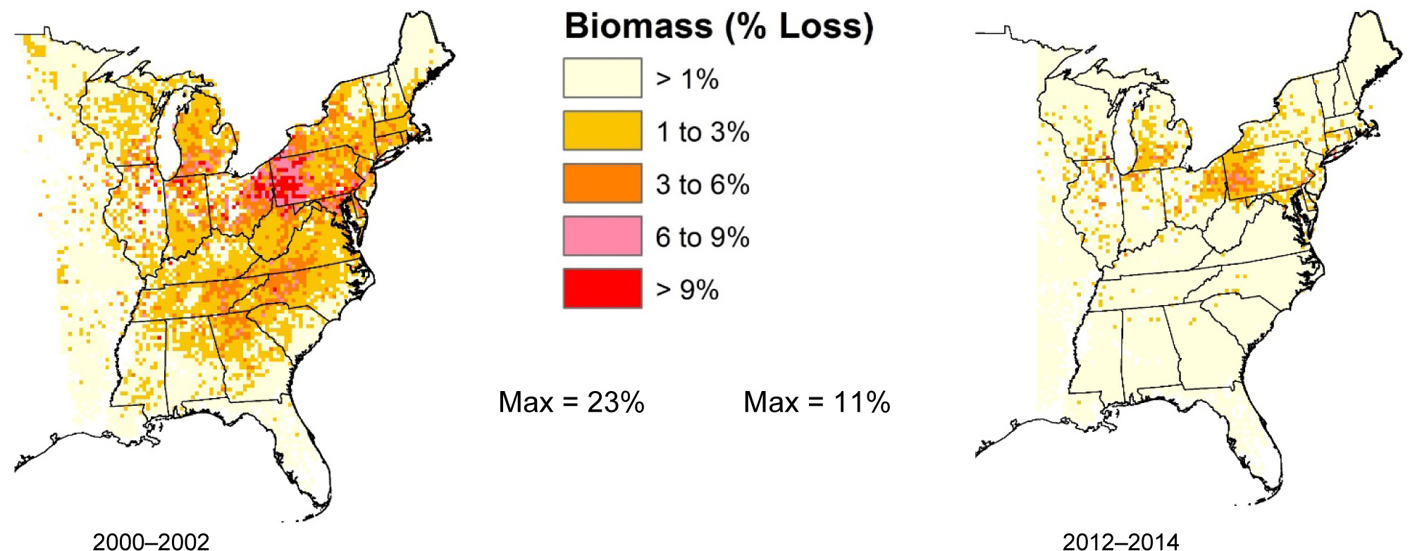 Download Figure
Source: Lynch et al., 2016
1 Areas with more than 2 percent biomass loss are defined here as significant based on a consensus workshop on O3 effects, which reported that a 2 percent annual biomass loss causes harm because of the potential for compounding effects over multiple years as short- term negative effects on seedlings affect long-term forest health (Heck and Cowling, 1997).
References
Amec Foster Wheeler Environment & Infrastructure, Inc. 2016a. Clean Air Status and Trends Network (CASTNET) First Quarter 2016 Data Summary. Prepared for U.S. Environmental Protection Agency (EPA), Office of Air and Radiation, Clean Air Markets Division, Washington, DC. Contract No. EP-W-16-015. Gainesville, FL.
Amec Foster Wheeler Environment & Infrastructure, Inc. 2016b. Clean Air Status and Trends Network (CASTNET) Fourth Quarter 2015 Data Report. Prepared for U.S. Environmental Protection Agency (EPA), Office of Air and Radiation, Clean Air Markets Division, Washington, DC. Contract No. EP-W-15-003. Gainesville, FL.
Amec Foster Wheeler Environment & Infrastructure, Inc. 2016c. Clean Air Status and Trends Network (CASTNET) Third Quarter 2015 Data Report. Prepared for U.S. Environmental Protection Agency (EPA), Office of Air and Radiation, Clean Air Markets Division, Washington, DC. Contract No. EP-W-15-003. Gainesville, FL.
Amec Foster Wheeler Environment & Infrastructure, Inc. 2015a. Clean Air Status and Trends Network (CASTNET) First Quarter 2015 Data Report. Prepared for U.S. Environmental Protection Agency (EPA), Office of Air and Radiation, Clean Air Markets Division, Washington, DC. Contract No. EP-W-15-003. Gainesville, FL.
Amec Foster Wheeler Environment & Infrastructure, Inc. 2015b. Clean Air Status and Trends Network (CASTNET) Second Quarter 2015 Data Report. Prepared for U.S. Environmental Protection Agency (EPA), Office of Air and Radiation, Clean Air Markets Division, Washington, DC. Contract No. EP-W-15-003. Gainesville, FL.
Amec Foster Wheeler Environment & Infrastructure, Inc. 2014. Clean Air Status and Trends Network (CASTNET) Quality Assurance Project Plan (QAPP) Revision 8.2. Prepared for U.S. Environmental Protection Agency (EPA), Office of Air and Radiation, Clean Air Markets Division, Washington, DC. Contract No. EP-W-09-028. Gainesville, FL. http://java.epa.gov/castnet/documents.do.
Baumann, K., Williams, E. J., Olson, J. A., Harder, J. W., and Fehsenfeld F. C. 1997. Meteorological Characteristics and Spatial Extent of Upslope Events during the 1993 Tropospheric OH Photochemistry Experiment. J. Geophys. Res., 102(D5), 6199–6213, doi:10.1029/96JD03251.
Butler, T., Vermeylen, F., Lehmann, C. M., Likens, G. E., and Puchalski, M. 2016. Increasing Ammonia Concentration Trends in Large Regions of the USA Derived from the NADP/AMoN Network. Atmos. Environ. 146, 132-140. doi: http://dx.doi.org/10.1016/j.atmosenv.2016.06.033.
Byun, D. and Schere, K. L. 2006. Review of the Governing Equations, Computational Algorithms, and Other Components of the Models‐3 Community Multiscale Air Quality (CMAQ) Modeling System. Applied Mechanics Reviews, 59: 51‐77. doi: 10.1115/1.2128636.
Camalier, L., Cox, W., and Dolwick, P. 2007. The Effects of Meteorology on Ozone in Urban Areas and their Use in Assessing Ozone Trends. Atmos Environ 41. 7127-7137.
Chappelka, A. H. and Samuelson L. J. 1998. Ambient Ozone Effects on Forest Trees of the Eastern United States: A Review. New Phytologist 139, 91 -108.
Edgerton, E., Walker, J., Chen, X., and Jansen, J. 2016. Measurements of NOy and HNO3 at a Rural-forested site in the Southern Appalachians. NADP Fall Science Meeting, Santa Fe, NM. http://nadp.sws.uiuc.edu/conf/2016/pptpdf/174_edgerton.pdf.
Environment Canada (ECAN) Water Science and Technology Directorate. 2015. Rain and Soft Waters PT Study 0106 Report. Proficiency Testing Program, Burlington, Ontario, Canada. Prepared for Amec Foster Wheeler Environment & Infrastructure, Inc., Newberry, FL, USA.
Environment Canada (ECAN) Water Science and Technology Directorate. 2016. Rain and Soft Waters PT Study 0107 Report. Proficiency Testing Program, Burlington, Ontario, Canada. Prepared for Amec Foster Wheeler Environment & Infrastructure, Inc., Newberry, FL, USA.
Heck, W. W. and Cowling, E. B. 1997. The Need for a Long-term Cumulative Secondary Ozone Standard–An Ecological Perspective, Environ. Management, (January) pp. 23-33.
International Organization for Standardization (ISO). 2005. Statistical Methods for the Use in Proficiency Testing by Interlaboratory Comparisons, Annex C, Robust Analysis, Section C.1: Algorithm A. Standard 13528. ISO 13528:2005(E).
Lavery, T. F., Rogers, C. M., Baumgardner Jr., R. E., and Mishoe, K. P. 2009. Intercomparison of CASTNET NO3- and HNO3 Measurements with Data from Other Monitoring Programs. J. Air & Waste Manage. Assoc., 59, 214-226.
Lefohn, A. S. and Runeckles, V. C. 1987. Establishing a Standard to Protect Vegetation – Ozone Exposure/Dose Considerations. Atmos. Environ., 21:561-568.
Li, Y., Schichtel, B. A., Walker J. T., Schwede, D. B., Chen, X., Lehmann, C. M., Puchalski, M. A., Gay, D. A., and Collett, J. L., Jr. 2016. Increasing Importance of Deposition in Reduced Nitrogen in the United States. Proc. of the National Academy of Sci. (113)21, 5874-5879. doi: http://dx.doi.org/10.1073/pnas.1525736113.
Lynch, J., Funk, C. S., Puchalski, M., and Haeuber, R. 2016. NOx Emissions Reductions Programs Have Translated to Improved Ozone Air Quality and Forest Health in the Eastern United States. The 7th International Nitrogen Initiative Conference (INI 2016), Melbourne, Australia. Accessed July 2017.
Martin, R. S. and Baasandorj, M. 2016. A Comparison of AMoN Measurements with Localized, Arrayed Passive NH3 Samplers in Northern Utah. Presentation submitted to the National Atmospheric Deposition Program (NADP), 2016 Fall Meeting, Santa Fe, NM.
McKernan, J., Dindal A., Kelly T., Hanft, E., and Cowen, K. 2011. Environmental Technology Verification Report and Statement for Applikon MARGA Semi-Continuous Ambient Air Monitoring System. U.S. Environmental Protection Agency, Washington, DC, EPA/600/R- 11/106, 2011. https://cfpub.epa.gov/si/si_public_record_report.cfm?dirEntryId=238475. Accessed September 2016.
National Science and Technology Council (NSTC). 2005. National Acid Precipitation Assessment Program Report to Congress: An Integrated Assessment. Executive Office of the President, National Science and Technology Council, Washington, DC. http://www.esrl.noaa.gov/csd/aqrs/reports/napapreport05.pdf. Accessed January 2017.
Ollinger, S. V., Aber, J. D., and Reich, P. B. 1997. Simulating Ozone Effects on Forest Productivity: Interactions, Among Leaf-canopy and Stand-level Processes. Ecological Applications 7(4) pp. 1237–1251.
Prasad, A. M. and Iverson, L. R. 2003. Little’s Range and FIA Importance Value Database for 135 Eastern U.S. Tree Species. Northeastern Research Station, USDA Forest Service. http://www.fs.fed.us/ne/delaware/4153/global/littlefia/index.html. Accessed January 2017.
Rumsey, I. C., Cowen, K. A., Walker, J. T., Kelly, T. J., Hanft, E. A., Mishoe, K., Rogers, C., Proost, R., Beachley, G. M., Lear, G., Frelink, T., and Otjes, R. P. 2014. An Assessment of the Performance of the Monitor for AeRosols and GAses in Ambient Air (MARGA): A Semi- Continuous Method for Soluble Compounds. Atmos. Chem. Phys., 14, 5639-5658, doi:10.5194/acp-14-5639-2014.
Schwab, J. J., Casson, P., Brandt, R., Husain, L., Dutkiewicz, V. A., Wolfe, D., Demerjian, K. L., Civerolo, K. L., Rattigan, O. V., Felton, D. H., and Dukett, J. E. 2016. Atmospheric Chemistry Measurements at Whiteface Mountain, NY: Cloud Water Chemistry, Precipitation Chemistry, and Particulate Matter. Aerosol and Air Quality Research, 16: 841–854, 2016 doi: 10.4209/aaqr.2015.05.0343.
Schwab, J. J., Wolfe, D., Casson, P., Brandt, R., Demerjian, K. L., Husain, L., Dutkiewicz, V. A., Civerolo, K. L., and Rattigan, O. V. 2016. Atmospheric Science Research at Whiteface Mountain, NY: Site Description and History. Aerosol and Air Quality Research, 16: 827–840, 2016 doi: 10.4209/aaqr.2015.05.0343.
Schwede, D. B. and Lear, G. G. 2014. A Novel Hybrid Approach for Estimating Total Deposition in the United States. Atmos. Environ., 92:207-220. doi: 10.1016/j.atmosenv.2014.04.008.
Sickles, J. E. and Shadwick, D. S. 2002. Biases in Clean Air Status and Trends Network Filter Pack Results Associated with Sampling Protocol. Atmos. Environ., 36(29):4687-4698. doi: 10.1016/S1352-2310(02)00405-3.
Slanina, J., ten Brink, H. M., Otjes, R. P., Even, A., Jongejan, P., Khlystov, A., Waijers-Ijpelaan, A., Hu, M., and Lu, Y. 2001. The Continuous Analysis of Nitrate and Ammonium in Aerosols by the Steam Jet Aerosol Collector (SJAC): Extension and Validation of the Methodology. Atmos. Environ. 35, 2319-2330.
Stein, A. F., Draxler, R. R, Rolph, G. D., Stunder, B. J. B., Cohen, M. D., and Ngan, F. 2015. NOAA’s HYSPLIT Atmospheric Transport and Dispersion Modeling System, Bull. Amer. Meteor. Soc., 96, 2059-2077, http://dx.doi.org/10.1175/BAMS-D-14-00110.1.
Talbot, R., Mao, H., and Sive, B. 2005. Diurnal Characteristics of Surface Level O3 and other Important Trace Gases in New England, J. Geophys. Res., 110, D09307, doi:10.1029/2004JD005449.
U. S. Environmental Protection Agency (EPA). 2016. Treatment of Data Influenced by Exceptional Events. http://www.epa.gov/ttn/analysis/exevents.htm. Accessed December 2014.
U. S. Environmental Protection Agency (EPA). 2015a. Title 40 Code of Federal Regulations (CFR) Appendix U to Part 50, Interpretation of the Primary and Secondary National Ambient Air Quality Standards for Ozone. https://www.ecfr.gov/cgi-bin/text- idx?SID=f69c175ad891728ce638989dfde88b85&mc=true&node=ap40.2.50_119.u&rgn=div9. Accessed September 2017.
U. S. Environmental Protection Agency (EPA). 2015b. Title 40 Code of Federal Regulations (CFR) Part 50, Primary and Secondary National Ambient Air Quality Standards. https://www.ecfr.gov/cgi-bin/text-idx?tpl=/ecfrbrowse/Title40/40cfr50_main_02.tpl. Accessed September 2017.
U. S. Environmental Protection Agency (EPA). 2015c. Total Deposition Estimates Using a Hybrid Approach. ftp://ftp.epa.gov/castnet/tdep/Total_Deposition_Documentation_current.pdf. Accessed June 2015.
U. S. Environmental Protection Agency (EPA). 2014a. National Emissions Inventory (NEI) Data. https://www.epa.gov/air-emissions-inventories/2014-national-emissions-inventory-nei-data Accessed March 27, 2017.
U. S. Environmental Protection Agency (EPA). 2014b. Welfare Risk and Exposure Assessment for Ozone Final. Office of Air and Radiation, Office of Air Quality Planning and Standards, Health and Environmental Impacts Division Risk and Benefits Group. Research Triangle Park, NC. EPA-452/R-14-005a https://nepis.epa.gov/Exe/ZyPDF.cgi?Dockey=P100KQ0H.txt Accessed July 2017.
U.S. Environmental Protection Agency (EPA) 2013. Title 40 CFR Appendix A to Part 58: Quality Assurance Requirements for Monitors used in Evaluations of National Ambient Air Quality Standards.
U. S. Environmental Protection Agency (EPA). 2008. National Ambient Air Quality Standards for Ozone; Final Rule. Federal Register 73, No. 60 (March). EPA-HQ-OAR-2005-0172.
U. S. Environmental Protection Agency (EPA). 2007. Review of the National Ambient Air Quality Standards for Ozone, Policy Assessment of Scientific and Technical Information. Office of Air Quality Planning and Standards Staff Paper. EPA-452/R-07-003. Available in Docket EPA- HQ-OAR-2003-0190 and at https://www.epa.gov/ttn/naaqs/standards/ozone/s_O3_cr_sp.html. Accessed January 2017.
Youden, W. J. (Ku, H. H., ed). 1969. Precision Measurement and Calibration. NBS Special Publication 300-Volume 1. U.S. Government Printing Office, Washington, DC.
Appendix A: Locational and Operational Characteristics of CASTNET Sites
| Site ID | Site Name | Start date | Latitude | Longitude | Elevation | Nearby NADP | Land Use | Terrain | Agency | Reference |
|---|---|---|---|---|---|---|---|---|---|---|
| ABT147, CT | Abington | 12/28/1993 | 41.8405 | -72.0104 | 202 | CT15 | Urban/Agric | Rolling | EPA | |
| ACA416, ME | Acadia NP | 12/1/1998 | 44.3771 | -68.2608 | 158 | ME98 | Forest | Rolling | NPS | |
| ALC188, TX | Alabama-Coushatta | 4/6/2004 | 30.7016 | -94.674 | 105 | TX10 | Prairie | Rolling | EPA | |
| ALH157, IL | Alhambra | 6/28/1988 | 38.869 | -89.6228 | 164 | IL46 | Agric | Flat | EPA | E |
| ANA115, MI | Ann Arbor | 6/28/1988 | 42.4166 | -83.9022 | 266 | MI52 | Forest | Flat | EPA | E |
| ARE128, PA | Arendtsville | 6/28/1988 | 39.9232 | -77.3079 | 266 | PA00 | Agric | Rolling | EPA | E |
| ASH135, ME | Ashland | 12/20/1988 | 46.6038 | -68.4132 | 231 | ME00 | Agric | Flat | EPA | E |
| BAS601, WY | Basin | 11/6/2012 | 44.28 | -108.0411 | 1242 | MT00 | Prairie | Rolling | BLM | |
| BBE401, TX | Big Bend NP | 7/18/1995 | 29.3027 | -103.1778 | 1052 | TX04 | Forest | Complex | NPS | W |
| BEL116, MD | Beltsville | 11/1/1988 | 39.0282 | -76.8171 | 47 | MD99 | Range | Flat | EPA | E |
| BFT142, NC | Beaufort | 12/28/1993 | 34.8847 | -76.6207 | 5 | NC06 | Agric | Flat | EPA | |
| BUF603, WY | Buffalo | 11/6/2012 | 44.1442 | -106.1089 | 1324 | WY99 | Prairie | Rolling | BLM | |
| BVL130, IL | Bondville | 2/9/1988 | 40.052 | -88.3725 | 213 | IL11 | Agric | Flat | EPA | E |
| BWR139, MD | Blackwater NWR | 7/4/1995 | 38.445 | -76.1113 | 1 | MD15 | Forest/ Marsh | Coastal | EPA | |
| CAD150, AR | Caddo Valley | 10/4/1988 | 34.1793 | -93.0988 | 78 | AR03 | Forest | Complex | EPA | E |
| CAN407, UT | Canyonlands NP | 1/24/1995 | 38.4583 | -109.8213 | 1809 | UT09 | Desert | Complex | NPS | W |
| CAT175, NY | Claryville | 5/10/1994 | 41.9423 | -74.552 | 754 | NY68 | Forest | Complex | EPA | |
| CDR119, WV | Cedar Creek | 11/10/1987 | 38.8795 | -80.8477 | 240 | WV05 | Forest | Complex | EPA | E |
| CDZ171, KY | Cadiz | 1/5/1999 | 36.7841 | -87.8502 | 190 | KY99 | Agric | Rolling | EPA | |
| CHA467, AZ | Chiricahua NM | 4/25/1989 | 32.0094 | -109.3891 | 1570 | AZ98 | Range | Complex | NPS | W |
| CHE185, OK | Cherokee Nation | 4/2/2002 | 35.7508 | -94.6698 | 305 | AR27 | Agric | Rolling | EPA | |
| CKT136, KY | Crockett | 8/24/1993 | 37.9215 | -83.0663 | 376 | KY35 | Agric | Rolling | EPA | |
| CND125, NC | Candor | 9/25/1990 | 35.2633 | -79.8375 | 172 | NC36 | Forest | Rolling | EPA | E |
| CNT169, WY | Centennial | 5/9/1989 | 41.3645 | -106.24 | 3175 | WY95 | Forest | Complex | EPA | W |
| COW005, NC | Coweeta Screwdriver Knob | 11/18/2014 | 35.0469 | -83.4531 | 960 | NC25 | Forest | Complex | EPA | |
| COW137, NC | Coweeta | 11/4/1987 | 35.0605 | -83.4303 | 683 | NC25 | Forest | Complex | EPA | E |
| CTH110, NY | Connecticut Hill | 9/29/1987 | 42.4009 | -76.6535 | 511 | NY67 | Forest | Rolling | EPA | E |
| CVL151, MS | Coffeeville | 12/27/1988 | 34.0027 | -89.7992 | 138 | MS30 | Forest | Rolling | EPA | |
| DCP114, OH | Deer Creek | 9/28/1988 | 39.6359 | -83.2606 | 264 | OH54 | Agric | Rolling | EPA | E |
| DEN417, AK | Denali NP | 10/6/1998 | 63.7232 | -148.9676 | 661 | AK03 | Forest | Complex | NPS | |
| DIN431, UT | Dinosaur NM | 11/20/2013 | 40.4373 | -109.3046 | 1463 | CO15 | Desert | Complex | NPS | |
| EGB181, ON | Egbert | 12/27/1994 | 44.2311 | -79.7831 | 227 | NY10 | Agric | Rolling | EPA | |
| ESP127, TN | Edgar Evins | 3/22/1988 | 36.0389 | -85.7331 | 302 | KY10 | Forest | Rolling | EPA | E |
| EVE419, FL | Everglades NP | 10/6/1998 | 25.3912 | -80.6808 | 2 | FL11 | Forest/ Marsh | Flat | NPS | |
| FOR605, WY | Fortification Creek | 5/21/2013 | 44.3395 | -105.9198 | 1408 | WY99 | Prairie | Rolling | BLM | |
| GAS153, GA | Georgia Station | 6/28/1988 | 33.1812 | -84.4101 | 265 | GA41 | Agric | Rolling | EPA | E |
| GLR468, MT | Glacier NP | 12/27/1988 | 48.5103 | -113.9968 | 976 | MT05 | Forest | Complex | NPS | W |
| GRB411, NV | Great Basin NP | 5/16/1995 | 39.0051 | -114.2159 | 2060 | NV05 | Forest | Complex | NPS | W |
| GRC474, AZ | Grand Canyon NP | 5/16/1989 | 36.0586 | -112.1836 | 2073 | AZ03 | Forest | Rolling | NPS | W |
| GRS420, TN | Great Smoky NP- Look Rock | 10/16/1998 | 35.6335 | -83.9416 | 793 | TN11 | Forest | Complex | NPS | |
| GTH161, CO | Gothic | 5/16/1989 | 38.9563 | -106.9859 | 2915 | CO10 | Range | Complex | EPA | W |
| HOW191, ME | Howland Ameriflux | 9/27/2011 | 45.204 | -68.74 | 68 | ME09 | Forest | Rolling | EPA | |
| HOX148, MI | Hoxeyville | 10/31/2000 | 44.1809 | -85.739 | 297 | MI53 | Forest | Flat | EPA | |
| HWF187, NY | Huntington Wildlife Forest | 5/28/2002 | 43.973 | -74.2233 | 497 | NY20 | Forest | Complex | EPA | |
| IRL141, FL | Indian River Lagoon | 7/9/2001 | 27.8492 | -80.4556 | 2 | FL99 | Coastal/ Marsh | Flat/ Water | EPA | |
| JOT403, CA | Joshua Tree NP | 2/16/1995 | 34.0696 | -116.3889 | 1244 | CA67 | Desert | Complex | NPS | W |
| KEF112, PA | Kane Experimental Forest | 1/3/1989 | 41.5981 | -78.7679 | 618 | PA29 | Forest | Rolling | EPA | E |
| KIC003, KS | Kickapoo Tribe | 2/18/2014 | 39.8539 | -95.6578 | 367 | KS97 | Prairie | Rolling | EPA | |
| KNZ184, KS | Konza Prairie | 3/26/2002 | 39.1022 | -96.6096 | 346 | KS31 | Prairie | Flat | EPA | |
| LAV410, CA | Lassen Volcanic NP | 7/25/1995 | 40.54 | -121.5765 | 1756 | CA96 | Forest | Complex | NPS | W |
| LRL117, PA | Laurel Hill | 12/15/1987 | 39.9883 | -79.2516 | 609 | PA83 | Forest | Complex | EPA | E |
| MAC426, KY | Mammoth Cave NP | 7/24/2002 | 37.1314 | -86.1481 | 243 | KY10 | Agric | Rolling | NPS | |
| MCK131, KY | Mackville | 7/31/1990 | 37.7047 | -85.0487 | 293 | KY03 | Agric | Rolling | EPA | E |
| MCK231, KY | Mackville Co-located | 12/29/1992 | 37.7047 | -85.0487 | 293 | KY03 | Agric | Rolling | EPA | |
| MEV405, CO | Mesa Verde NP | 1/10/1995 | 37.1984 | -108.4905 | 2165 | CO99 | Forest | Complex | NPS | W |
| MKG113, PA | M.K. Goddard | 1/12/1988 | 41.4268 | -80.1452 | 377 | NY10 | Forest | Rolling | EPA | E |
| NEC602, WY | Newcastle | 11/7/2012 | 43.873 | -104.1919 | 1468 | WY99 | Prairie | Rolling | BLM | |
| NIC001, NY | Nicks Lake | 11/20/2012 | 43.6805 | -74.9891 | 525 | NY29 | Forest | Rolling | NYSDEC | |
| NPT006, ID | Nez Perce Tribe | 12/15/2015 | 46.2756 | -116.0216 | 945 | Forest | Rolling | EPA | ||
| OXF122, OH | Oxford | 8/18/1987 | 39.5311 | -84.7235 | 284 | OH09 | Agric | Rolling | EPA | E |
| PAL190, TX | Palo Duro SP | 4/24/2007 | 34.8806 | -101.6647 | 1053 | TX02 | Prairie | Complex | EPA | |
| PAR107, WV | Parsons | 1/19/1988 | 39.0904 | -79.6617 | 510 | WV18 | Forest | Complex | EPA | E |
| PED108, VA | Prince Edward | 11/3/1987 | 37.1652 | -78.3071 | 149 | VA24 | Forest | Rolling | EPA | E |
| PET427, AZ | Petrified Forest | 9/12/2002 | 34.8225 | -109.8925 | 1723 | AZ97 | Desert | Flat | NPS | |
| PIN414, CA | Pinnacles NM | 5/16/1995 | 36.4832 | -121.1569 | 335 | CA66 | Forest | Complex | NPS | W |
| PND165, WY | Pinedale | 12/27/1988 | 42.929 | -109.7878 | 2386 | WY06 | Forest | Rolling | EPA | W |
| PNF126, NC | Cranberry | 12/27/1988 | 36.1054 | -82.045 | 1216 | NC45 | Forest | Mountain-top | EPA | E |
| PRK134, WI | Perkinstown | 9/27/1988 | 45.2065 | -90.5972 | 462 | WI35 | Agric | Rolling | EPA | E |
| PSU106, PA | Penn State | 1/6/1987 | 40.7209 | -77.9318 | 364 | PA42 | Agric | Rolling | EPA | E |
| QAK172, OH | Quaker City | 1/5/1999 | 39.9427 | -81.3379 | 371 | OH49 | Agric | Rolling | EPA | |
| RED004, MN | Red Lake Nation | 8/26/2014 | 47.8638 | -94.8352 | 372 | MN16 | Forest | Flat | EPA | |
| ROM206, CO | Rocky Mountain NP Co-located | 7/3/2001 | 40.2781 | -105.5456 | 2742 | CO19 | Forest | Complex | EPA | |
| ROM406, CO | Rocky Mountain NP | 12/20/1994 | 40.2781 | -105.5456 | 2743 | CO19 | Forest | Complex | NPS | W |
| SAL133, IN | Salamonie Reservoir | 6/28/1988 | 40.816 | -85.6614 | 250 | IN20 | Agric | Flat | EPA | E |
| SAN189, NE | Santee Sioux | 7/5/2006 | 42.8292 | -97.8541 | 434 | SD99 | Range | Rolling | EPA | |
| SEK430, CA | Sequoia & Kings Canyon NP - Ash Mountain | 4/7/2005 | 36.4895 | -118.8292 | 510 | CA75 | Forest | Mountain-top | NPS | |
| SHE604, WY | Sheridan | 11/6/2012 | 44.93 | -106.85 | 1115 | MT00 | Prairie | Rolling | BLM | |
| SHN418, VA | Shenandoah NP - Big Meadows | 6/28/1988 | 38.5231 | -78.4347 | 1073 | VA28 | Forest | Mountain-top | NPS | E |
| SND152, AL | Sand Mountain | 12/27/1988 | 34.289 | -85.9701 | 349 | AL99 | Agric | Rolling | EPA | E |
| SPD111, TN | Speedwell | 6/12/1989 | 36.4698 | -83.8265 | 361 | TN04 | Agric | Rolling | EPA | E |
| STK138, IL | Stockton | 12/28/1993 | 42.2872 | -90 | 281 | IL18 | Agric | Rolling | EPA | |
| SUM156, FL | Sumatra | 12/27/1988 | 30.1102 | -84.9904 | 16 | FL23 | Forest | Flat | EPA | E |
| THR422, ND | Theodore Roosevelt NP | 10/6/1998 | 46.8948 | -103.3777 | 850 | ND00 | Forest | Rolling | NPS | |
| UND002, VT | Underhill | 11/13/2012 | 44.5283 | -72.8688 | 399 | VT99 | Forest | Complex | EPA | |
| UVL124, MI | Unionville | 6/28/1988 | 43.6136 | -83.3599 | 202 | MI51 | Agric | Flat | EPA | E |
| VIN140, IN | Vincennes | 8/4/1987 | 38.7408 | -87.4849 | 136 | IN22 | Agric | Rolling | EPA | E |
| VOY413, MN | Voyageurs NP | 6/13/1996 | 48.4125 | -92.8292 | 429 | MN32 | Forest | Rolling | NPS | |
| VPI120, VA | Horton Station | 6/2/1987 | 37.3298 | -80.5575 | 920 | VA13 | Agric | Mountain-top | EPA | E |
| WFM007, NY | Whiteface Mountain Summit | 6/4/2015 | 44.36608 | -73.90312 | 1415 | NY98 | Forest | Complex | EPA | |
| WFM105, NY | Whiteface Mountain | 11/20/2012 | 44.39 | -73.86 | 570 | NY98 | Forest | Complex | NYSDEC | |
| WNC429, SD | Wind Cave NP | 11/20/2003 | 43.5576 | -103.4839 | 1292 | SD04 | Prairie | Rolling | NPS | |
| WSP144, NJ | Washington Crossing | 12/27/1988 | 40.3123 | -74.8727 | 59 | NJ99 | Range | Rolling | EPA | E |
| WST109, NH | Woodstock | 12/27/1988 | 43.9445 | -71.7008 | 255 | NH02 | Forest | Complex | EPA | E |
| YEL408, WY | Yellowstone NP | 6/26/1996 | 44.5654 | -110.4003 | 2400 | WY08 | Agric | Rolling | NPS | W |
| YOS404, CA | Yosemite NP - Turtleback Dome | 9/25/1995 | 37.7133 | -119.7062 | 1605 | CA99 | Forest | Complex | NPS | W |
Note:
NM = National Monument
NP = National Park
NWR = National Wildlife Reserve
SP = State Park
E = eastern reference site
W = western reference site
Appendix B: Acronyms and Abbreviations
| A2LA | American Association for Laboratory Accreditation |
| Amec Foster Wheeler | Amec Foster Wheeler Environment & Infrastructure, Inc. |
| AMNet | Atmospheric Mercury Network |
| AMoN | Ammonia Monitoring Network |
| AQS | EPA's Air Quality System |
| ARP | Acid Rain Program |
| ASRC | Atmospheric Sciences Research Center |
| BLM | Bureau of Land Management |
| C-R | concentation-response |
| Ca | particulate calcium |
| CAAA | Clean Air Act Amendments |
| CAMx | Comprehensive Air Quality Model with Extensions |
| CAPMoN | Canadian Air and Precipitation Monitoring Network |
| CASTNET | Clean Air Status and Trends Network |
| CFR | Code of Federal Regulations |
| Cl- | particulate chloride |
| CMAQ | Community Multiscale Air Quality Modeling System |
| CO | carbon monoxide |
| CSAPR | Cross-State Air Pollution Rule |
| DM8A | daily maximum 8-hour average |
| DQI | data quality indicator |
| ECAN | Environment Canada |
| EGUs | electric generating units |
| EPA | U.S. Environmental Protection Agency |
| Hg | mercury |
| HNO | nitric acid |
| HONO | nitrous acid |
| HYSPLIT | Hybrid Single Particle Lagrangian Integrated Trajectory model |
| IEC | International Electrotechnical Commission |
| IMPROVE | Interagency Monitoring of Protected Visual Environments |
| ISO | International Organization for Standardization |
| K | particulate potassium |
| kg ha yr | kilograms per hectare per year |
| km | kilometer |
| m | meter |
| MADPro | Mountain Acid Deposition Program |
| MARGA | Monitor for Aerosols and Gases in Ambient Air |
| MARPD | mean absolute relative percent difference |
| MCCP | Mountain Cloud Chemistry Project |
| MDL | method detection limit |
| MDN | Mercury Deposition Network |
| Mg | particulate magnesium |
| mg/L | milligrams per liter |
| MRPD | mean relative percent difference |
| MU | MARGA unit |
| N | nitrogen |
| Na | particulate sodium |
| NAAQS | National Ambient Air Quality Standards |
| NADP | National Atmospheric Deposition Program |
| NAPAP | National Acid Precipitation and Assessment Program |
| NCore | EPA's National Core Monitoring |
| NH | ammonia |
| NH | particulate ammonium |
| NHNO | ammonium nitrate |
| NO | nitrogen oxide |
| NO | nitrogen dioxide |
| NO | particulate nitrate |
| NOx | nitrogen oxides [nitrogen oxide (NO) + nitrogen dioxide (NO)] |
| NOy | total reactive oxides of nitrogen |
| NOz | HNO, nitrous oxide, peroxyacetyl nitrate, peroxyproyl nitrate, other organic nitrates, and nitrite |
| NPS | National Park Service |
| NTN | National Trends Network |
| NYSDEC | New York State Department of Environmental Conservation |
| O | ozone |
| PFA | pulsed fluorescence analyzer |
| PM | particulate matter |
| PM2.5 | fine particulate matter |
| ppb | parts per billion |
| ppm | parts per million |
| PRISM | Parameter-elevation Regressions on Independent Slopes Model |
| PT | proficiency testing |
| QA | quality assurance |
| QAPP | Quality Assurance Project Plan |
| QC | quality control |
| R2 | coefficient of determination |
| S | sulfur |
| SCR | selective catalytic reduction |
| SEARCH | Southeastern Aerosol Research and Characterization Network |
| SO | sulfur dioxide |
| SO | particulate sulfate |
| TDEP | NADP Total Deposition Hybrid Method |
| total NO | gaseous nitric acid (HNO) + particulate nitrate (NO) |
| TSP | total suspended particles |
| USDA | U.S. Department of Agriculture |
| µeq/L | microequivalents per liter |
| µg/m | micrograms per cubic meter |
| WARMS | Wyoming Air Resources Monitoring System |