Executive Summary
The EPA Clean Air Status and Trends Network (CASTNET) measures concentrations of atmospheric pollutants across the United States. The primary objectives of the network are to provide data to evaluate the effectiveness of national and regional air pollution control programs, to determine compliance with ozone National Ambient Air Quality Standards, to improve estimates of dry and total deposition, and to improve the calculation and mapping of critical loads of sulfur and nitrogen to terrestrial ecosystems. CASTNET data are also used to provide input to the National Atmospheric Deposition Program’s Total Deposition Hybrid Method for calculating total deposition and for regional air quality model evaluation. This report presents 2014 maps of ozone levels, nitrogen and sulfur pollutant concentrations, and deposition fluxes and examines trends in air quality over the 25-year period from 1990 through 2014. In 2014, CASTNET measured rural, regionally representative concentrations of nitrogen and sulfur species at 93 monitoring stations in 91 locations and ozone levels at 80 locations.
Key Results and Highlights through 2014
The mean fourth highest daily maximum 8-hour average (DM8A) ozone (O3) concentration for 2014 at eastern CASTNET reference sites (see Appendix A for designated reference sites) was 63 parts per billion (ppb) or, equivalently, 0.063 parts per million (ppm), the lowest in the history of the network. At the western reference sites, the value was 65 ppb. Three-year averages of fourth highest DM8A O3 concentrations exceeded the 2008 National Ambient Air Quality Standard (NAAQS) of 0.075 ppm at three California CASTNET sites during the most recent 3-year period (2012–2014). No eastern sites measured exceedances. Three-year averages of fourth highest DM8A O3 concentrations were reduced by 22 percent at the eastern reference sites since 1990–1992 and by 6 percent at the western reference sites since 1996–1998. Figure E-1 and Table E-1 summarize the long-term changes in measured concentrations. During 2014, three CASTNET sites, all in California, measured fourth highest DM8A O3 concentrations greater than 0.075 ppm.
Three-year mean annual concentrations of total nitrate (NO3-), which is comprised of nitric acid (HNO3) plus particulate NO3-, declined 44 percent at eastern sites over the 25-year period. Over the same period, nitrogen oxides (NOx) emissions were reduced by 78 percent at regulated electric generating units (EGUs) in the East. Three-year mean annual total NO3- levels measured at western reference sites dropped by 27 percent over the 19-year period.
Mean annual sulfur dioxide (SO2) concentrations measured at eastern reference sites have declined significantly over the 25-year period 1990 through 2014. Three-year mean annual SO2 levels at eastern sites declined 82 percent. The percent reduction in SO2 concentrations at CASTNET eastern reference sites (82 percent) is consistent with the reduction in regulated eastern EGU SO2 emissions (80 percent). SO2 concentrations measured at western reference sites declined by 50 percent over the 19 years from 1996 through 2014.
Table E-1 Trends in Aggregated Western and Eastern O3, Total NO3-, and SO2 Pollutant Concentrations
| Pollutant | Western Sites | Eastern Sites | Percent Changed | |||
|---|---|---|---|---|---|---|
| 1996-98 | 2012-14 | 1990-92 | 2012-14 | West | East | |
| O3 (ppb) | 74 | 69 | 85 | 66 | -6 | -22 |
| Total NO3- (μg/m 3) | 1.0 | 0.7 | 3.0 | 1.7 | -27 | -44 |
| SO2 (μg/m 3) | 0.6 | 0.3 | 3.0 | 1.7 | -50 | -82 |
The original focus of CASTNET was to measure pollutant concentrations for estimating long-term trends in sulfur and nitrogen pollutants. Recently, the focus has changed to include demonstrating compliance of rural, regional O3 concentrations with the NAAQS. The network also added measurements of trace-level gases and speciated nitrogen pollutants. Additionally, CASTNET supports the Ammonia Monitoring Network (AMoN) with operation of ammonia samplers at or near 65 CASTNET sites.
This report provides information on CASTNET pollutant measurements and estimated deposition fluxes. It also presents information on special topics such as maps of critical loads for the United States.
Chapter 1: CASTNET Update
The Clean Air Status and Trends Network (CASTNET) performs long-term monitoring of air pollutant concentrations in rural areas across the United States to determine compliance with ozone National Ambient Air Quality Standards and to evaluate the effectiveness of national and regional emission control programs. CASTNET is also operated to identify trends in rural atmospheric ozone, nitrogen, and sulfur concentrations and deposition fluxes of nitrogen and sulfur pollutants. CASTNET data are used to provide input to the National Atmospheric Deposition Program’s Total Deposition Hybrid Method and for regional air quality model evaluation. CASTNET is managed and operated by the U.S. Environmental Protection Agency (EPA) in cooperation with the National Park Service and other federal, state, and local partners. CASTNET was established under the 1990 Clean Air Act Amendments, expanding the National Dry Deposition Network, which began in 1987. In 2014, the network operated 93 monitoring stations throughout the contiguous United States, Alaska, and Canada. CASTNET measurements are needed to provide accountability for EPA emission control programs and to assess their effectiveness. CASTNET data demonstrate the continuing reductions in ozone, nitrogen, and sulfur pollutant concentrations, which have declined significantly over the last 25 years.
Introduction
The Acid Rain Program (ARP) was established by the U.S. Congress under Title IV of the 1990 Clean Air Act Amendments (CAAA). The ARP was enacted to reduce emissions of sulfur dioxide (SO2) and nitrogen oxides (NOx) from electric generating units (EGUs) and has produced significant reductions in emissions since 1995. Since then, other air pollution control programs have been instituted to reduce emissions of SO2 and NOx. For example, the Clean Air Interstate Rule (CAIR) was enacted in 2005 to reduce emissions in 27 eastern states and the District of Columbia. Earlier control programs include the 1990 Ozone Transport Commission NOx Budget Program, the 1998 NOx State Implementation Plan (SIP) Call, and the 2003 NOx Budget Trading Program (NBP). The emission reductions achieved under these programs have resulted in a dramatic improvement in air quality as demonstrated by air pollutant concentrations measured by CASTNET and other cooperating networks. By 2014, EGUs required to comply with ARP/CAIR had reduced their SO2 emissions to about 3.2 million tons and NOx emissions to about 1.7 million tons, decreases of 80 and 73 percent, respectively, from 1990 levels.
On July 6, 2011, the Cross-State Air Pollution Rule (CSAPR) was promulgated to require 28 states in the eastern half of the United States to significantly improve air quality by reducing EGU emissions that cross state lines and contribute to ground level ozone (O3) and fine particle (PM2.5) pollution in other states. It was designed to reduce annual SO2, annual NOx, and O3 season NOx emissions while providing sources with flexibility in how to comply with the program. CSAPR was intended to replace CAIR starting in 2012, but, due to various court actions, implementation of CSAPR was delayed. CSAPR Phase 1 implementation and CASTNET 2014 Annual Report 2 Chapter 1: CASTNET Update compliance began in January 2015. EPA (2016) updated CSAPR on September 7, 2016 to address interstate transport of O3 with respect to the 2008 O3 National Ambient Air Quality Standard (NAAQS; EPA, 2008). Phase 2 compliance will begin in 2017.
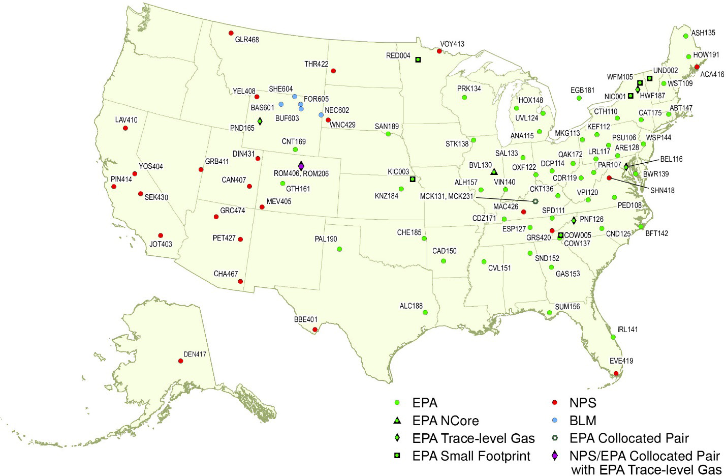
Congress mandated in the 1990 CAAA that the EPA provide consistent, long-term measurements for determining relationships between changes in emissions and subsequent changes in air quality, atmospheric deposition, and ecological effects. CASTNET operated 93 monitoring stations in 2014 throughout the contiguous United States, Alaska, and Canada. EPA and the National Park Service (NPS) are the primary sponsors of CASTNET. NPS began its participation in 1994 and operated 25 sites during 2014. The Bureau of Land Management (BLM) operated five sites in Wyoming.
In 2014, small footprint sites were added to tribal lands for the Kickapoo Tribe in Kansas (KIC003) and the Red Lake Band of Chippewa Indians in Minnesota (RED004). A small footprint site that uses solar and wind energy sources for power was installed at Coweeta (Screwdriver Knob), NC (COW005).
This report summarizes CASTNET monitoring and the resulting concentration and deposition data collected over the 25-year period from 1990 through 2014. Additional information, previous annual reports, other CASTNET documents, and the CASTNET database can be found on the EPA CASTNET website, https://www.epa.gov/castnet/. The website provides a complete archive of concentration and deposition data for all CASTNET sites.
Cooperating Networks
CASTNET monitors air quality and deposition in cooperation with other national and international networks. EPA uses CASTNET and these other long-term national networks to assess the effectiveness of emission control programs.
National Atmospheric Deposition Program (NADP) operates:
- National Trends Network (NTN), which includes about 260 monitoring stations with wet deposition samplers to measure the concentrations and deposition rates of air pollutants removed from the atmosphere by precipitation. NTN operates wet deposition samplers at or near every CASTNET site.
- Ammonia Monitoring Network (AMoN), which operates passive ammonia (NH3) samplers at about 92 sites with about 65 of the AMoN sites at or near CASTNET locations. AMoN, in operation since 2007, provides 2-week integrated NH3 concentrations.
- Mercury Deposition Network (MDN), which operates samplers to measure mercury (Hg) in precipitation. MDN samplers are operated at several CASTNET sites.
- Atmospheric Mercury Network (AMNet), which measures atmospheric concentrations of gaseous oxidized, particulate-bound, and elemental Hg at about 20 locations in the continental United States, Canada, Hawaii, and Taiwan in order to estimate dry and total Hg deposition.
NADP’s website gives detailed information on each of these sub-networks.
Canadian Air and Precipitation Monitoring Network (CAPMoN) operates 33 measurement sites throughout Canada and 1 in the United States. CASTNET and CAPMoN both operate filter pack samplers in Ontario, Canada. CAPMoN operates a wet deposition sampler at the Pennsylvania State University CASTNET site (PSU106, PA).
EPA’s National Core Monitoring (NCore) reports on particulate matter (PM) mass; PM species; O3, SO2, nitrogen oxide/total reactive oxides of nitrogen (NO/NOy), and carbon monoxide (CO) concentrations; and meteorological parameters at approximately 80 sites.
BLM’s Wyoming Air Resources Monitoring System (WARMS) operates eight sites and the meteorological system at Pinedale (PND165), one of the EPA-sponsored CASTNET sites, in Wyoming. Five of the WARMS sites are CASTNET-protocol sites.
Interagency Monitoring of Protected Visual Environments (IMPROVE) measures speciated aerosol pollutants that affect visibility near more than 20 CASTNET sites. Visit the IMPROVE website for more information.
Locations of Monitoring Sites
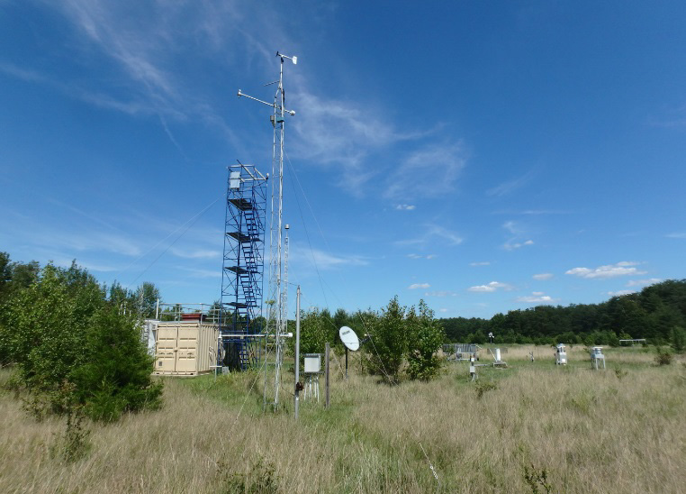
The locations of the CASTNET monitoring sites that were operational during 2014 are depicted in Figure 1-1. Ninety-three monitoring sites were operated at 91 distinct locations. To estimate precision across the network, collocated sites were operated at Mackville, KY (MCK131/231) and Rocky Mountain National Park, CO (ROM406/206) during 2014. The ROM406/206 pair ensures consistency between EPA (ROM206) and NPS (ROM406) operations. MCK131 and ROM406 are specified as the regulatory monitoring sites for O3. Appendix A provides the location of each site by state and includes information on start date, latitude, longitude, elevation, identification of the nearby NADP site, land use, terrain type, operating agency, and if the site is a reference site used for trends. Three new sites (KIC003, KS; RED004, MN; and COW005, NC) were added to the network during 2014.
Measurements Recorded at CASTNET Sites
All CASTNET sites measure weekly ambient concentrations of acidic pollutants, base cations, and chloride (Cl -) using a 3-stage filter pack with a controlled flow rate (Amec Foster Wheeler, 2013). Gaseous pollutant measurements include SO2 and nitric acid (HNO3). Particulate concentrations include sulfate (SO42-), nitrate (NO3-), ammonium (NH4+ ), magnesium (Mg 2+), calcium (Ca 2+), potassium (K +), sodium (Na +), and Cl -. The filter pack is exchanged each Tuesday and shipped to the Amec Foster Wheeler analytical chemistry laboratory in Gainesville, FL for analysis. Ambient temperature is measured at 9-meters (m) at all sites in part to enable conversion of concentrations to local conditions.
Most CASTNET sites also include a temperature-controlled shelter and continuous O3 monitoring system. The O3 inlet and filter pack are located atop a 10-m tower. Some CASTNET sites also measure trace-level SO2, CO, and NO/NOy. In 2014, meteorological parameters were measured at 6 EPA-, 25 NPS-, and 5 BLM-sponsored CASTNET sites. Measured meteorological parameters include 2-m temperature, wind speed and direction, standard deviation of the wind direction, solar radiation, relative humidity, precipitation, and surface wetness.
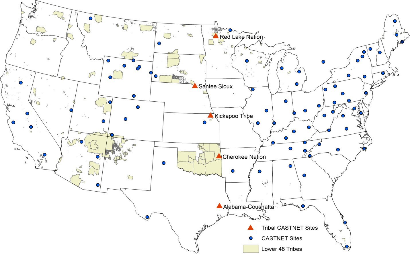
Building Tribal Partnerships with CASTNET Monitoring Sites
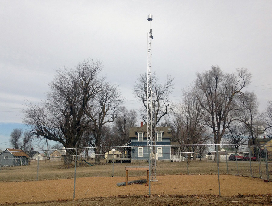
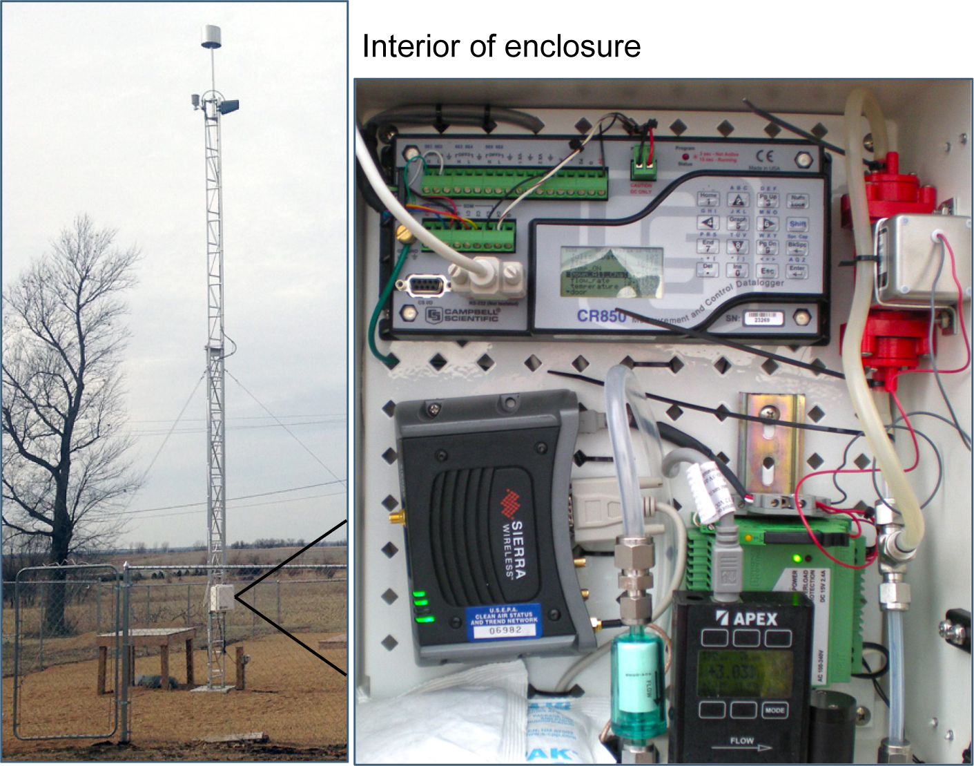
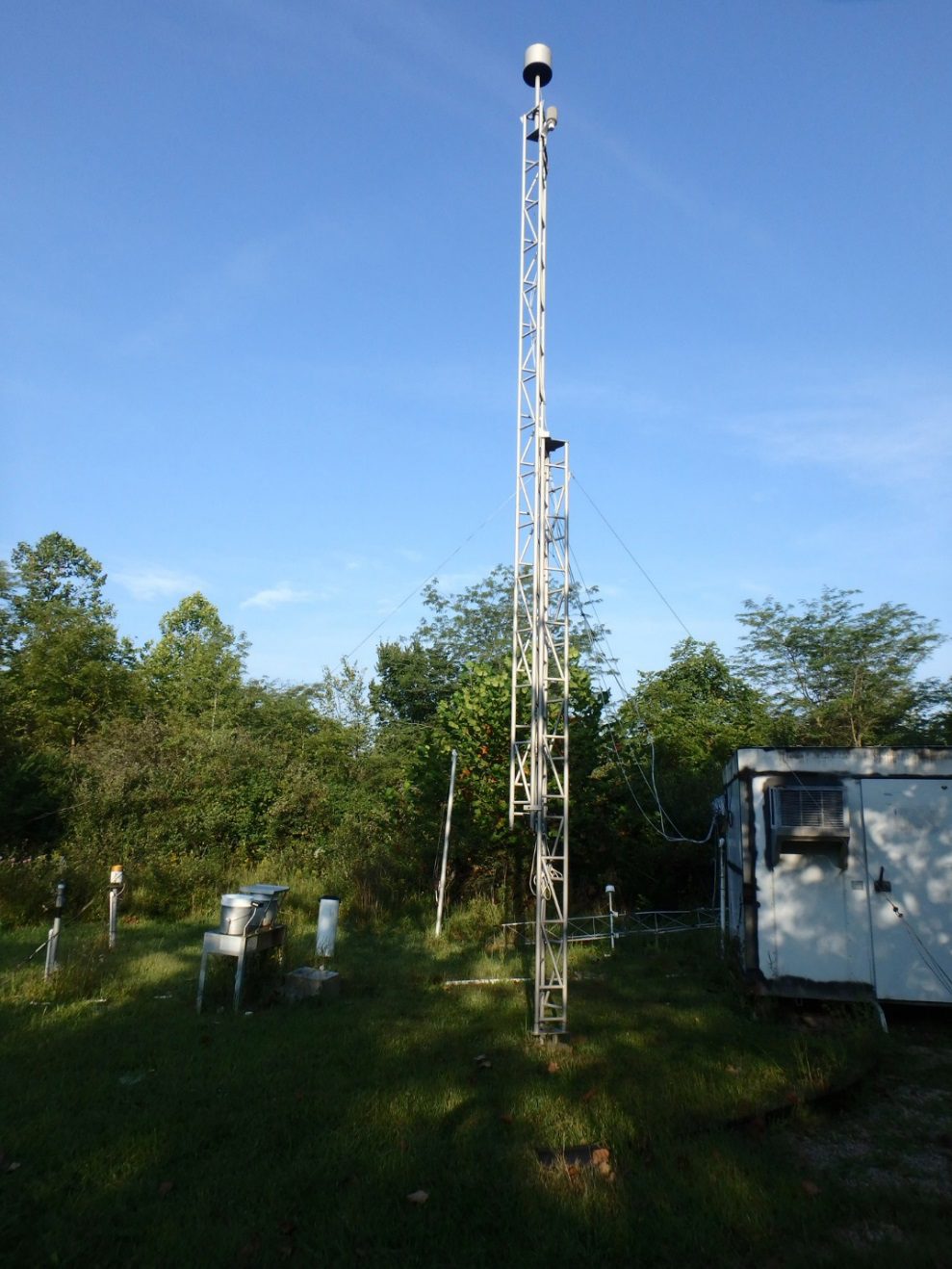
EPA partners with Cherokee Nation, OK (2002); the Alabama-Coushatta Tribe, TX (2004); the Santee Sioux Tribe, NE (2006); the Kickapoo Tribe in Kansas (2014); and the Red Lake Band of Chippewa Indians in Minnesota (2014) to operate CASTNET sites on tribal lands. In 2012, CASTNET developed a small footprint monitoring station that does not require a temperaturecontrolled shelter. The new type of monitoring station includes a 10-m sampling tower, 3-stage filter pack, pump, flow meter, data logger, and cellular modem (Figure 1-2). The new site design has produced cost savings and increased efficiency in terms of installation and power. The advent of the small footprint monitoring station has opened opportunities for new partners, such as the Kickapoo Tribe in Kansas and the Red Lake Band of Chippewa Indians, to participate in the CASTNET monitoring program. EPA may support additional tribal groups that are interested in establishing small footprint sites.
The operation of CASTNET monitoring sites on tribal lands provides benefits to both the tribes and EPA. The CASTNET measurements provide data on atmospheric pollutants and deposition fluxes to areas important to tribes. The measurements help the tribes understand the environmental effects of prescribed burns, wild fires, and nearby point or urban sources.
For EPA, partnerships are important for operating a consistent, stable, long-term monitoring network. Current tribal sites fill in spatial gaps in the network within the central United States (Figure 1-3), and tribes provide much needed support for operations and infrastructure. Many sites operate collocated monitoring instruments on behalf of NCore, NADP, MDN, AMNet, and AMoN. The Cherokee Nation, Alabama-Coushatta, and Santee Sioux tribal sites provide regulatory O3 data to AIRNow and EPA’s Air Quality System (AQS).
Kickapoo Tribe, KS (KIC003)
Estimating Dry, Wet, and Total Deposition
Total deposition was assessed using the NADP’s Total Deposition Hybrid Method (EPA, 2015b; Schwede and Lear, 2014), which is a hybrid approach that combines data from established ambient monitoring networks and large scale models. To estimate dry deposition, ambient measurement data from CASTNET and other networks were merged with dry deposition rates and flux output from the Community Multiscale Air Quality (CMAQ) modeling system. Wet deposition estimates were derived from precipitation chemistry measurements and precipitation amounts from the Parameter-elevation Regressions on Independent Slopes Model (PRISM). Dry and wet deposition fluxes were added to obtain the estimates of total deposition that are discussed in Chapters 9, 10, and 11.
Quality Assurance Program
The CASTNET Quality Assurance (QA) program was designed to ensure that all reported data are of known and documented quality in order to meet CASTNET objectives. The QA program was established to ensure intra-network consistency and comparability and to deliver data that are reproducible and comparable with data from other monitoring networks and laboratories. The 2014 QA program elements are documented in the CASTNET Quality Assurance Project Plan (QAPP; Amec Foster Wheeler, 2013). The QAPP includes standards and policies for all components of project operation from site selection through final data reporting with appendices that provide standard operating procedures for CASTNET operations.
Data quality indicators (DQI) such as precision, accuracy, and completeness are used to assess CASTNET measurements and supporting activities. Routine assessment and analysis help guarantee the production of high-quality data and information to meet project objectives. Measurements taken during 2014 and historical data collected over the period 1990 through 2013 were analyzed relative to DQI and their associated metrics. Results from these analyses are available in quarterly and annual QA reports posted on the EPA CASTNET website. Selected analyses are summarized in callout boxes labeled, “QA Program Summary,” where appropriate throughout this report.
QA Program Summary
Laboratory Intercomparison Results
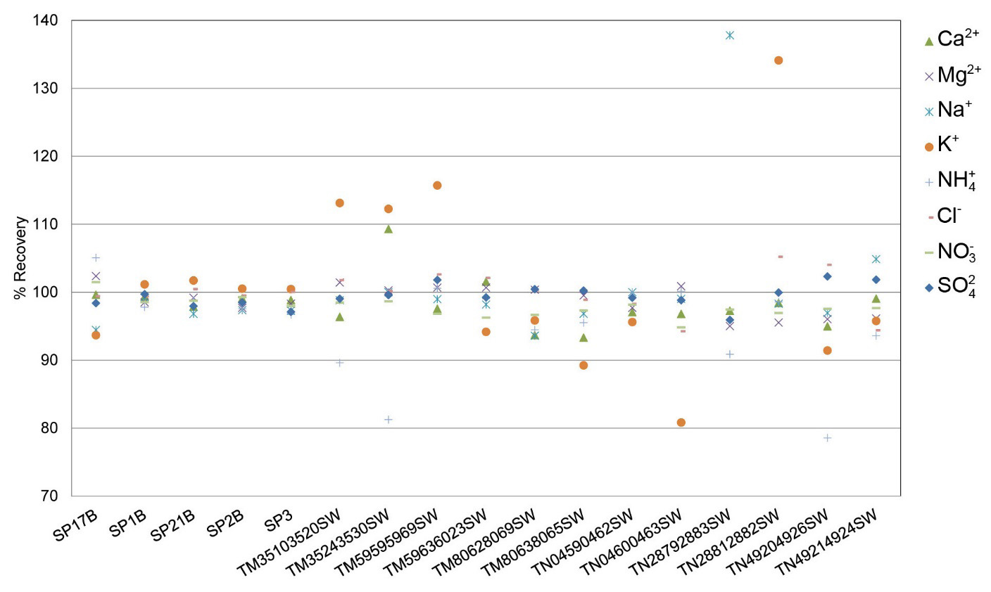
The Amec Foster Wheeler laboratory is one of eight laboratories that participated in the U.S. Geological Survey (USGS) interlaboratory comparison program in 2014. The USGS external QA programs are designed to facilitate integration of data from various monitoring networks that routinely measure atmospheric deposition by estimating the variability and bias of analytical results determined by the separate laboratories. The laboratory receives 48 samples from the USGS for chemical analysis and reporting during the course of each year. The number of samples received for 2014 totaled 40 due to a lost shipment. The 2014 samples were a mix of 13 standard reference samples with certified National Institute of Standards and Technology (NIST)-traceable values prepared by High Purity Standards, which were diluted and spiked by the USGS; 3 deionized water samples; and 24 excess natural wet deposition samples collected at NADP sites and prepared by the USGS or the NADP Central Analytical Laboratory. Several replicates of similar concentration levels are received each year.
Results for the eight CASTNET parameters for the synthetically prepared and natural samples are depicted in Figure 1-a. The named samples in the figure are grouped by verified concentration level. Seventeen distinct groups are represented. Results are presented as percent recoveries of the median value for all laboratories – defined as the most probable value (MPV). The MPV calculation excludes values below laboratory quantitation limits. One hundred twenty-four of 134 mean sample values were within 10 percent of their corresponding MPV. The 10 values exceeding 10 percent of their MPV were obtained from natural samples.
Chapter 2: Ozone Concentrations
CASTNET is the primary network for monitoring ground-level ozone concentrations at rural sites in the United States. It produces critical information on geographic patterns in rural ozone levels. Ozone data measured at CASTNET sites are submitted to EPA’s Air Quality System. CASTNET ozone data from 2012 through 2014 were evaluated with respect to the National Ambient Air Quality Standards (EPA, 2008). Maps of 3-year averages of fourth highest daily maximum 8-hour average (DM8A) ozone concentrations for 2012 through 2014 and fourth highest DM8A ozone concentrations for 2014 are presented. Trends in fourth highest DM8A ozone concentrations for eastern and western reference sites are shown using box plots.
Most CASTNET sites operate an O3 analyzer that measures hourly average concentrations, which are presented on the CASTNET website and reported in the AQS. During 2014, 80 O3 analyzers were operated throughout the network. Data from these sites, with the exception of Howland, ME (HOW191) and the collocated sites at MCK231, KY and ROM206, CO, which are designated as non-regulatory, are used to calculate fourth highest DM8A concentrations annually. Three-year averages (design values) are calculated when three years of Title 40 Code of Federal Regulations (CFR) Part 58-compliant data become available. CASTNET’s geographic coverage of the United States provides data that are essential for evaluating rural O3 concentrations in the context of the O3 NAAQS and in terms of presenting information on trends and geographic patterns in regional O3.
A design value is a statistic that describes the air quality status of a given area relative to the concentration values required by the NAAQS. Design values change as each new 3-year data set of monitored ozone concentrations becomes available. Design values are used to classify nonattainment areas, assess progress towards meeting the NAAQS, and develop control strategies to achieve the NAAQS. For example, if 3-year averages of 2012–2014 fourth highest DM8A ozone concentrations are used for purposes of attainment designation and exceed 0.075 parts per million (ppm), then ozone concentrations would have to be reduced to 0.075 ppm or below to achieve the 2008 ozone NAAQS. Official criteria pollutant nonattainment area and county information are provided on the EPA website.
The information presented in this chapter includes maps of and trends in the annual fourth highest DM8A O3 concentrations measured at CASTNET sites. Additional maps of O3 concentrations from the NPS Air Atlas can be viewed at nature.nps.gov.
Measurements from 34 CASTNET eastern and 16 western reference sites (see Appendix A) were analyzed to determine trends in O3 concentrations. The reference sites were also used to show trends in ambient nitrogen and sulfur concentrations (Chapters 3 and 7). The 34 eastern sites have been reporting CASTNET measurements since at least 1990 and the 16 western sites since at least 1996. The site at Mount Rainier National Park, WA (MOR409), which was a western reference site, was terminated in September 2013.
National Ambient Air Quality Standards for Ozone
Ozone Standards for 2008 and 2015
| Ozone 1 | Year | Primary Standard | Secondary Standard | |
|---|---|---|---|---|
|
Level |
Averaging Time |
Level |
Averaging Time |
|
|
2008 |
0.075 ppm 1 |
8-hour 2 |
0.075 ppm 1 |
8-hour 2 |
|
2015 |
0.070 ppm 1 |
8-hour 3 |
0.070 ppm 1 |
8-hour 3 |
Note:
1 The NAAQS was revised from 0.075 ppm to 0.070 ppm on October 1, 2015.
2 To attain the 2008 standard, the 3-year average of the fourth highest DM8A O3 concentrations measured at each monitor within a specified area must not exceed 0.075 ppm or 75 parts per billion (ppb) in practice (effective May 27, 2008; EPA, 2008). O3 concentrations are commonly presented in units of ppb.
3 To attain the 2015 standard, the 3-year average of the fourth highest DM8A O3 concentrations measured at each monitor within a specified area must not exceed 0.070 ppm or 70 ppb in practice (effective October 1, 2015; EPA, 2015a).
The primary O3 NAAQS is designed to protect public health. The secondary standard is designed to protect public welfare and the environment. Both O3 NAAQS are set at a level of 0.075 ppm averaged over eight hours for the annual fourth highest daily maximum value averaged across three consecutive years.
Revised Standards
On November 25, 2014, EPA proposed to update both the primary and secondary standards for O3. Both standards would have been 8-hour standards set within a range of 0.065 to 0.070 ppm. On October 1, 2015, EPA (2015a) revised the primary and secondary NAAQS to a level of 0.070 ppm. EPA retained the pollutant indicator (O3), forms (fourth highest daily maximum averaged across three consecutive years), and averaging time (eight hours; EPA, 2015a). The 2015 standard includes some changes to how 8-hour concentrations are calculated and other administrative changes. The secondary standard is equivalent, based on the W126 index, to a level of protection of 17 ppm-hour or lower averaged over three years (EPA, 2015a). The W126 index is a seasonal measure often used to assess the impact of O3 exposure on ecosystems and vegetation including crop production.
The EPA and other federal, tribal, state, and local agencies measure O3 concentrations on an hourly basis through national and local monitoring programs. Amec Foster Wheeler followed EPA procedures (1998) to estimate O3 design values and annual fourth highest DM8A O3 concentrations at CASTNET sites. Measurements potentially affected by exceptional events were not removed when calculating these estimates. “Exceptional events 1 are unusual or naturally occurring events that can affect air quality but are not reasonably controllable using techniques that state, tribal, or local air agencies may implement in order to attain and maintain the NAAQS” (EPA, 2013b). Potential exceptional events are reported to the EPA by state/local monitoring agencies. Data possibly affected are flagged in the AQS until a final demonstration package is accepted or rejected by the EPA.
CASTNET O3 data for the years 2012 through 2014 are used to gauge compliance with the NAAQS at EPA- and NPS-sponsored sites that have been operated under regulatory QA procedures. The BLM WARMS O3 sites are compliant operationally with 40 CFR Part 58 requirements but currently have insufficient information to calculate 3-year averages of the fourth highest DM8A O3 concentrations.
Quality Assurance Program Results
Ozone Concentrations
Ozone quality control (QC) criteria are set forth in 40 CFR Part 58, Appendix A (EPA, 2013a). Figure 2-a presents summary statistics of critical criteria O3 measurements at EPA-sponsored CASTNET sites collected during 2014. All data associated with QC checks that fail to meet the established criteria were invalidated unless the cause of failure was documented to have no effect on ambient data collection. QC failures for EPA-sponsored sites are addressed in quarterly QA reports, which can be found on the EPA CASTNET website.
Note:
QA program results for NPS-sponsored sites measuring O3 may be accessed here.
1 A revised Exceptional Events Rule was posted for public comment on 9/16/2016.
Eight-Hour Ozone Concentrations
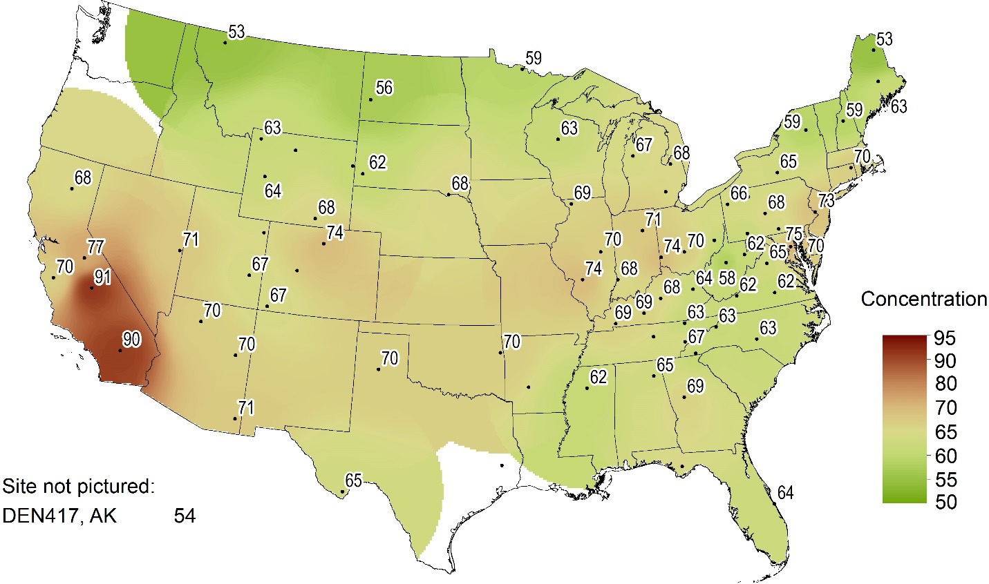
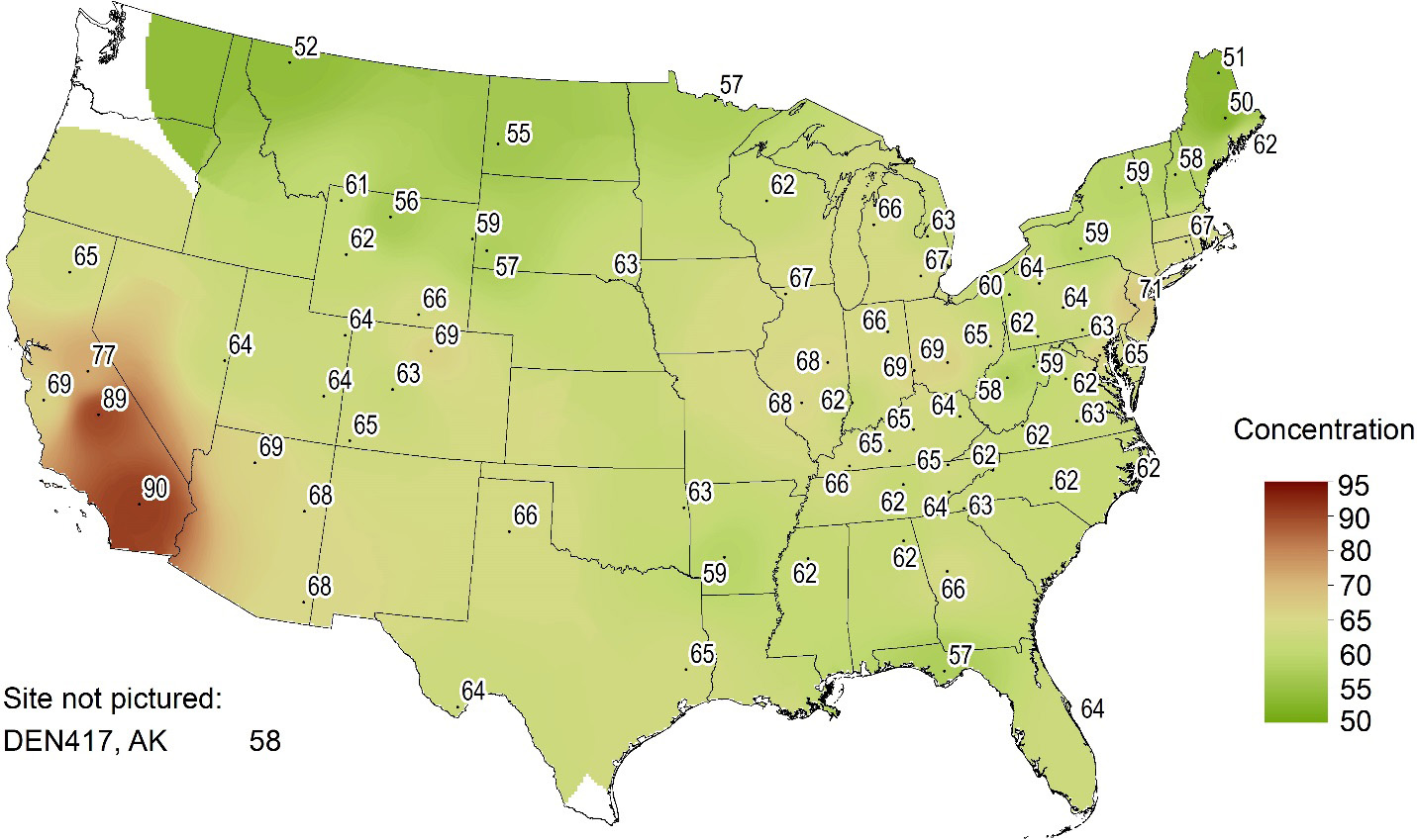
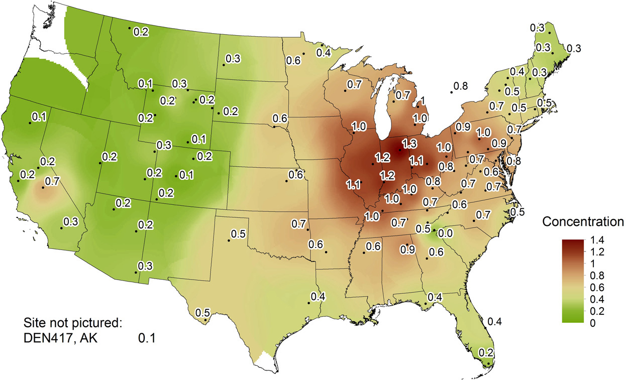
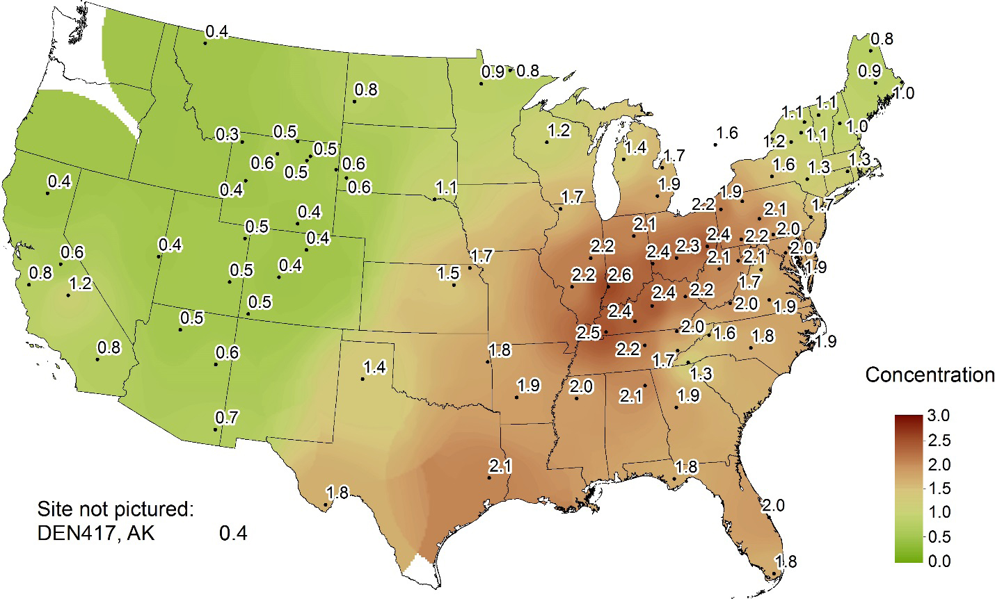
All CASTNET O3 data for 2012 through 2014 were measured at sites with regulatory designated monitors (except for HOW191, ME; MCK231, KY; and ROM206, CO) and, therefore, were used to calculate fourth highest DM8A O3 concentrations and to gauge compliance with the NAAQS. Data for HOW191 are shown on the maps in this chapter for informational purposes only. Figure 2-1 presents 3-year averages of the fourth highest DM8A O3 concentrations for 2012 through 2014. O3 concentrations were not included if the 3-year average was not available because of incomplete data; these sites are shown as dots with no value. Three California CASTNET sites measured fourth highest DM8A O3 concentrations above the 0.075 ppm NAAQS. The highest western O3 concentration of 91 ppb was sampled at Sequoia National Park, CA (SEK430). The highest eastern concentration of 75 ppb was measured at Beltsville, MD (BEL116).
Figure 2-1 Three-year Average of Fourth Highest DM8A O3 Concentrations (ppb) for 2012–2014
 Download Image
All valid 2014 O3 concentrations that meet completeness requirements are shown in Figure 2-2. During 2014, no eastern CASTNET sites measured O3 concentrations greater than 75 ppb. Three California CASTNET sites measured concentrations above 75 ppb. The highest DM8A concentration for 2014 was 90 ppb measured at Joshua Tree National Park, CA (JOT403).
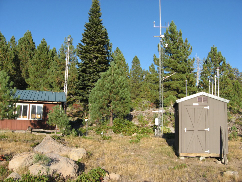
Joshua Tree National Park, CA (JOT403)
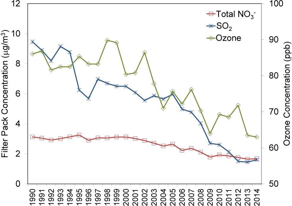
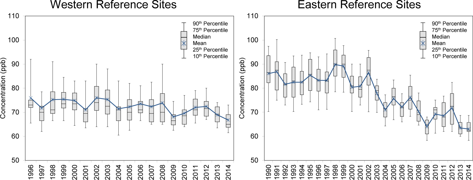
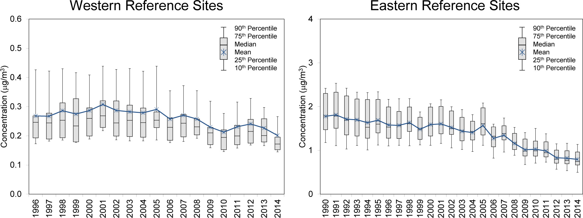
Figure 2-3 provides box plots depicting trends in 1-year mean values and annual distributions of fourth highest DM8A O3 concentrations from the 34 CASTNET eastern reference sites (right side) for 1990 through 2014 and for the 16 western reference sites (left side) for 1996 through 2014. The eastern O3 data show an overall decrease since 1998. The 2014 aggregate median data point, 63 ppb, is the lowest level for the eastern reference sites in the history of the network.
The western O3 data show an increase in fourth highest DM8A O3 concentrations from 2009 through 2012, followed by a decrease in 2013 and 2014. The 2014 median of the fourth highest DM8A O3 concentrations for the western reference sites was 65 ppb. Similar to the statistics for the eastern reference sites, the 2014 median value for the western reference sites is the lowest in the history of the network.
Chapter 3: Nitrogen Pollutant Concentrations
Weekly average concentrations of nitric acid, particulate nitrate, and particulate ammonium were measured using 3-stage filter packs at 93 CASTNET monitoring stations during 2014. Trends in mean annual total nitrate (nitric acid plus nitrate) and ammonium concentrations were aggregated over 34 eastern and 16 western reference sites and are shown using box plots. The nitrogen pollutants measured at the 34 eastern reference sites decreased over the 25-year period from 1990 through 2014. Concentrations of total nitrate began to drop in 2000 in response to nitrogen oxides emission reduction mandates and have continued to decrease slowly with a 44 percent reduction from 1990 through 2014. Total nitrate and ammonium concentrations measured at the 16 western reference sites declined over the 19-year period 1996 through 2014.
Maps of 2014 annual mean concentrations of total NO3- (HNO3 + NO3-) and NH4+ are presented in this chapter. Additional maps of 2014 quarterly mean concentrations are provided in CASTNET quarterly data reports (Amec Foster Wheeler, 2014a; 2014b; 2015b; 2015c). Trends in annual mean concentrations over the 25-year period (1990 through 2014) were derived from measurements from the 34 CASTNET eastern reference sites and for the period 1996 through 2014 from data measured at 16 CASTNET western reference sites. See Appendix A for the designated reference sites.
Total Nitrate Concentrations
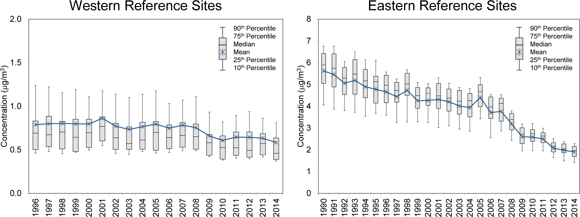
Mean total NO3- concentrations measured in 2014 are presented on the map in Figure 3-1. To illustrate trends, Figure 3-2 provides box plots of total NO3- levels for the eastern and western reference sites through 2014. Each box presents the mean and median concentrations and the 10th, 25th, 75th, and 90th percentiles for that year. The data shown on the right side of the figure were aggregated from the 34 eastern reference sites. The data show no trend in mean concentrations until 2000 when total NO3- levels began to decline in response to NOx emission control programs. Total NO3- levels measured at the eastern reference sites were reduced from a mean value of 3.1 micrograms per cubic meter (μg/m 3 ) of air in 2000 to a mean value of 1.7 μg/m3 in 2014. Over the history of the network, 3-year mean levels declined from 3.0 μg/m 3 for 1990–1992 to 1.7 μg/m 3 for 2012–2014, producing a 44 percent reduction in total NO3-. The 2014 mean concentration was slightly higher than the 2013 level of 1.6 μg/m 3 .
The left side of Figure 3-2 shows data aggregated from the 16 western sites. The 3-year mean total NO3- concentration for 2012–2014 was 27 percent lower than the corresponding 1996–1998 level. The 3-year mean concentration was 1.0 μg/m 3 for 1996–1998 and 0.7 μg/m 3 for 2012–2014.
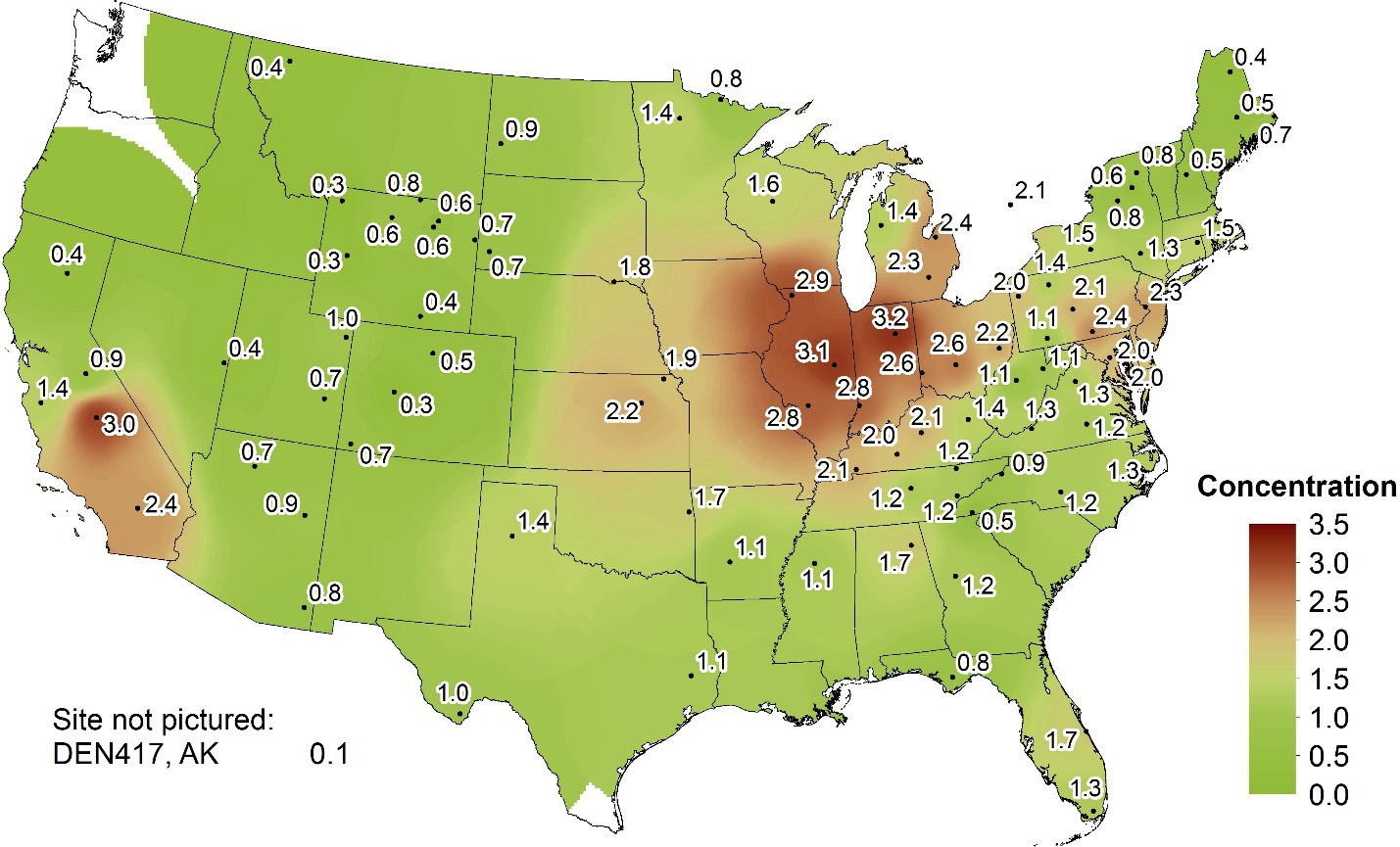
Total nitrate concentrations measured at the 34 eastern sites declined by 44 percent. Total nitrate levels measured at the western reference sites were reduced by 27 percent. Total nitrate concentrations measured at the eastern sites were generally two to three times higher than concentrations measured at western reference sites.
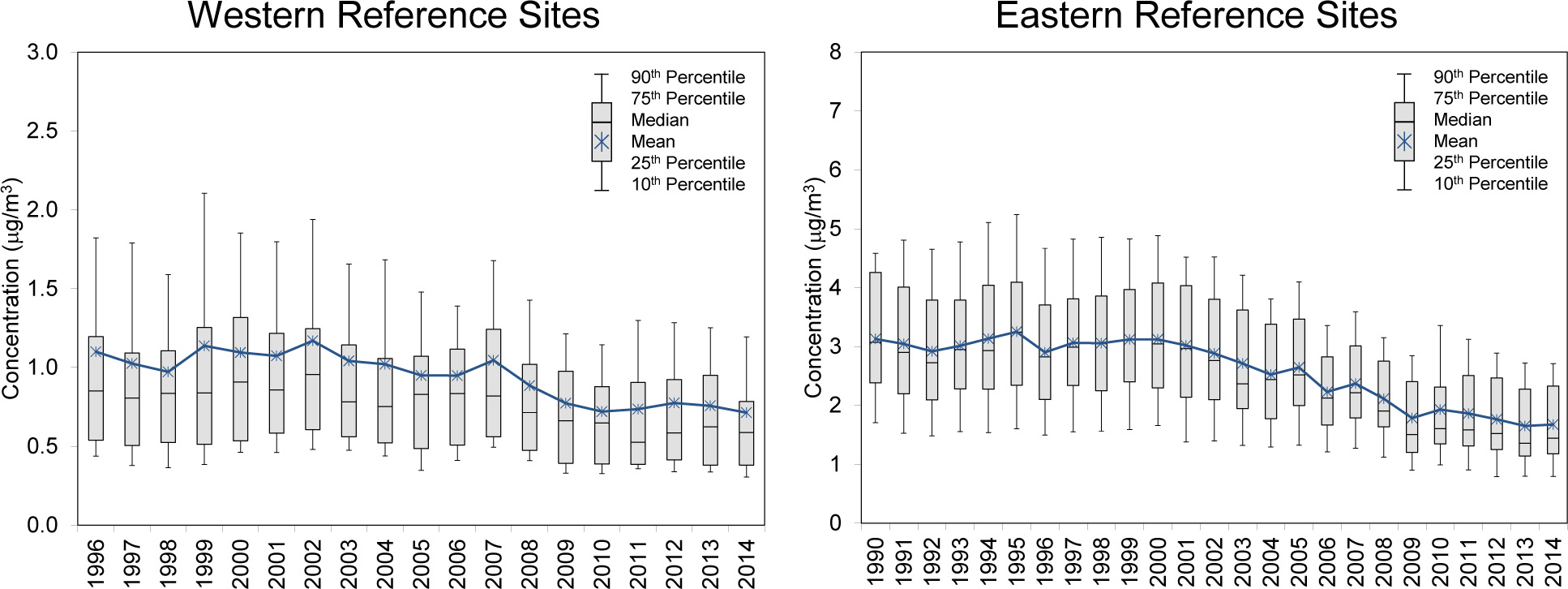
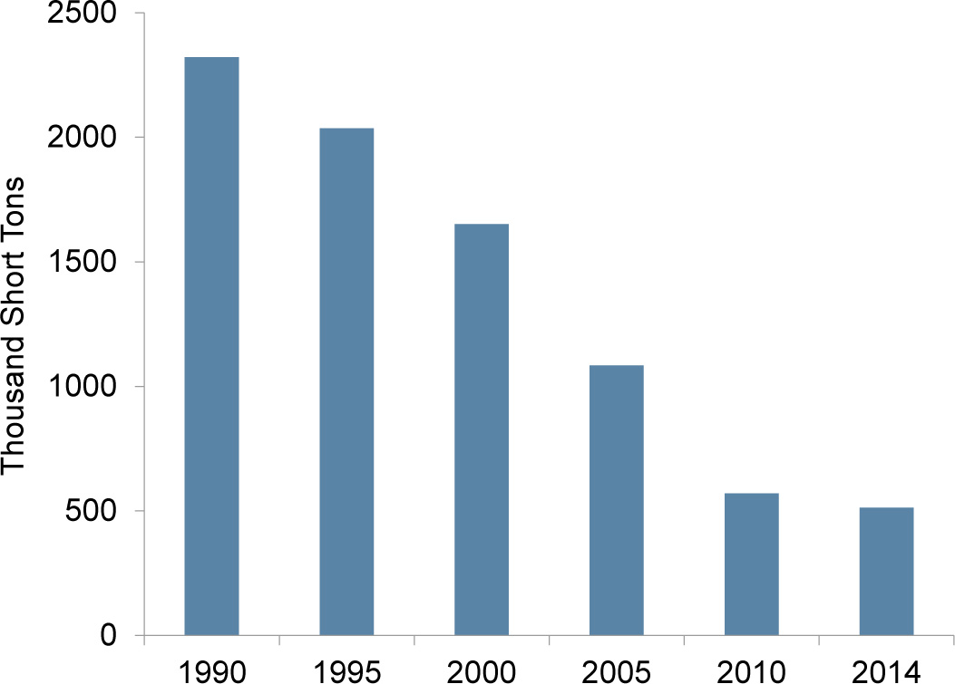
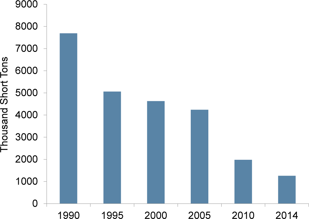
Figure 3-3 illustrates the trend in NOx emissions from regulated EGUs operating in the eastern United States from 1990 through 2014. The 25-year decline in aggregated EGU emissions was 78 percent.
Figure 3-3 Trend in Annual Composite NOx Emissions from Regulated EGUs Operating in Illinois, Indiana, Kentucky, Ohio, Pennsylvania, and West Virginia
 Download Image
Particulate Ammonium Concentrations
A map of 2014 mean particulate NH4+ concentrations is provided in Figure 3-4. Figure 3-5 shows box plots of NH4+ concentrations. The trend diagram for the eastern sites (right side) shows a reduction in mean NH+ 4 levels from 1990–1992 to 2012–2014. The 1990–1992 mean concentration was 1.8 μg/m 3 , and the 2012–2014 value was 0.8 μg/m 3 , a 53 percent decline. The western reference sites show a decline from 0.3 μg/m 3 in 1996–1998 to 0.2 μg/m 3 in 2012–2014, an 18 percent reduction.
Quality Assurance Program Results
Precision of Filter Pack Measurements
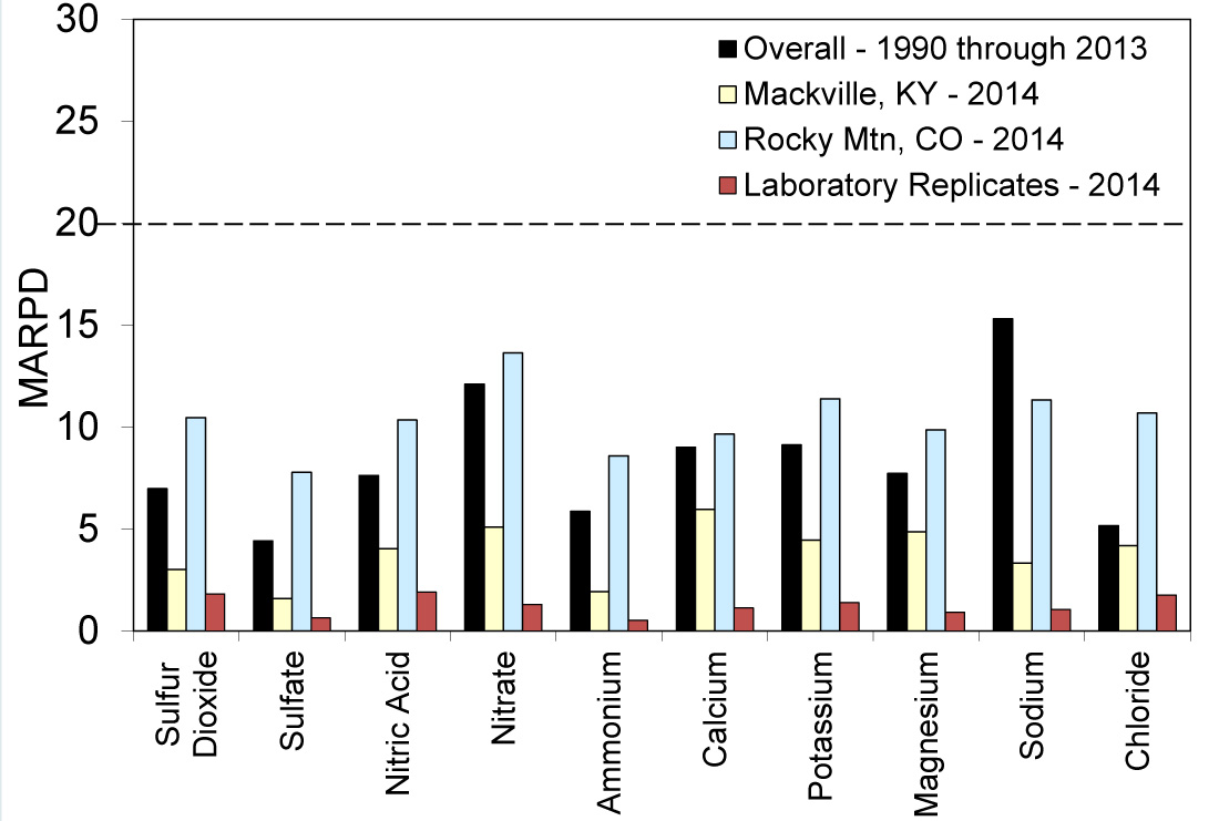
Historical (1990 through 2013) mean absolute relative percent difference (MARPD) data for all 11 collocated site pairs operated over the history of the network are provided in the bar chart in Figure 3-a. The 2014 data for the current collocated sites at MCK131/231, KY and ROM406/206, CO are also provided. The precision criterion is a MARPD of 20 percent. Historical and 2014 measurements met the criterion for each analyte.
Figure 3-a Historical and 2014 Precision Results for Atmospheric Concentrations and Laboratory Replicate Samples
 Download Image
The 2014 analytical precision results for 10 measurements are presented in Figure 3-a. The results were based on analysis of 5 percent of the samples that were randomly selected for replication in each batch. The results of in-run replicate analyses were compared with the original concentration results. The laboratory precision data met the 20 percent measurement criterion by a large margin. All MARPD values for laboratory replicates were less than 2 percent.
Data Completeness
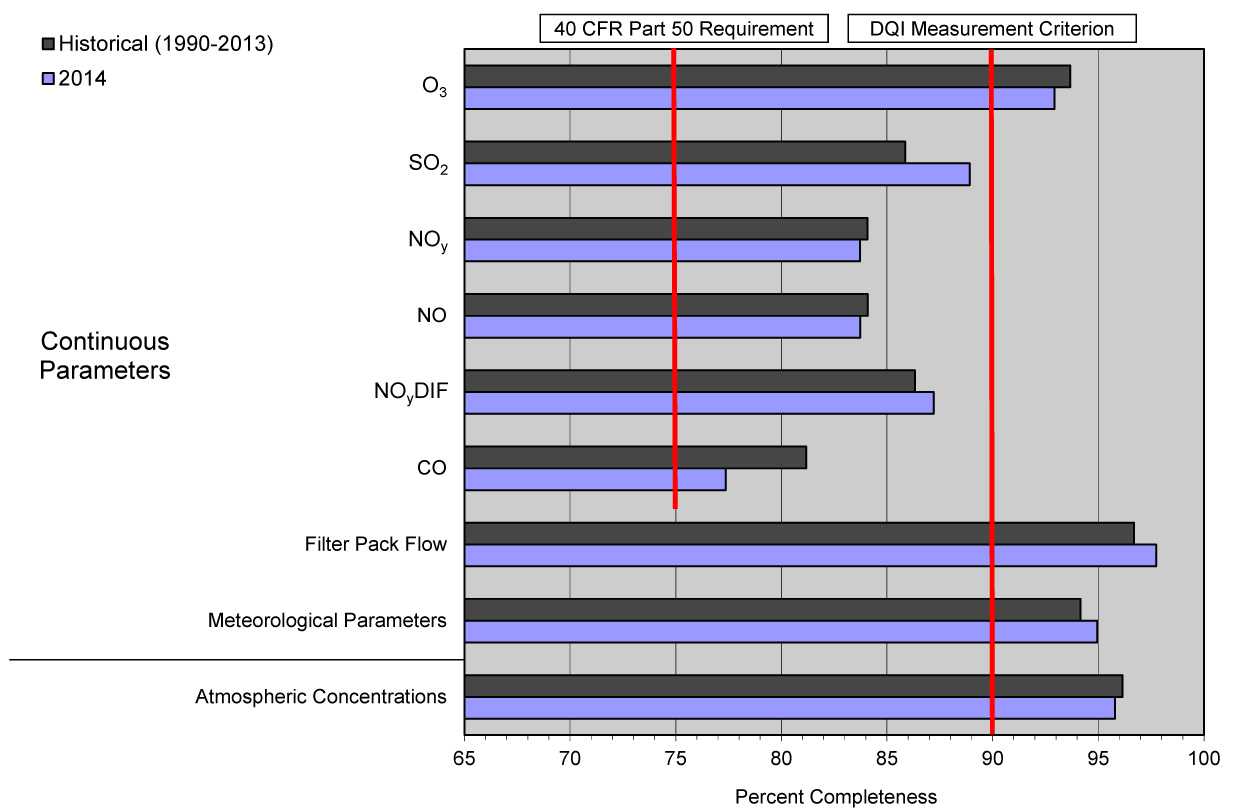
Completeness is defined as the percentage of valid data points obtained from a measurement system relative to total possible data points. The CASTNET measurement criterion for completeness requires a minimum completeness of 90 percent for every measurement for each quarter. The historical results and the results for 2014 are given in Figure 3-b. Historical results for trace-level gas measurements represent data from 2013. The completeness criterion was met for atmospheric (filter pack) and O3 concentrations, filter pack flow, and meteorological measurements. Completeness of trace-level gas measurements (Chapter 4) met the completeness requirements of 40 CFR Part 50 (EPA, 2013a).
Figure 3-b Historical and 2014 Percent Completeness of Measurements (black bars are 1990–2013 for long-term data and for 2013 for trace-level gas data)
 Download Image
Chapter 4: Continuous Trace-level Gas Concentrations
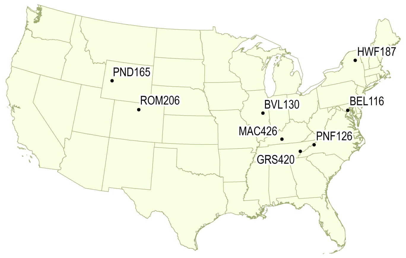
Continuous trace-level gas air quality monitors were operated at eight CASTNET sites during 2014. EPA sponsored six of the monitors and NPS two. The measurements at these sites were performed to (1) support EPA NCore monitoring, (2) provide data to understand atmospheric processes such as ozone and fine particulate matter formation, and (3) generate data for regional model input and evaluation. Total reactive oxides of nitrogen was measured at all eight sites, sulfur dioxide at three sites, and carbon monoxide at two sites. Total reactive oxides of nitrogen concentrations were highest at the suburban Maryland site and lowest at the high-elevation, mountainous sites.
Continuous trace-level gas analyzers were deployed at six EPA and two NPS CASTNET sites during 2014. Table 4-1 lists the site locations, start dates, and the trace-level gas parameters measured at each site. These data were sampled continuously and archived as 1-hour values. In addition to these CASTNET measurements, NO/NOy monitors were operated by other federal and state agencies at CASTNET or nearby sites in North Dakota, South Dakota, and Maine.
Table 4-1 Continuous Trace-level Gas Monitoring Sites Operated during 2014
| Site Location | Start Date | Measurements |
|---|---|---|
| Beltsville, MD (BEL116) | March 2005 | NO/NOy and SO2 |
| Mammoth Cave National Park, KY (MAC426)* | May 2009 | NO/NOy, SO2, and CO |
| Bondville, IL (BVL130) | July 2012 | NO/NOy, SO2, and CO |
| Huntington Wildlife Forest, NY (HWF187) | November 2012 | NO/NOy |
| Pinedale, WY (PND165) | May 2013 | NO/NOy |
| Cranberry, NC (PNF126) | October 2013 | NO/NOy |
| Rocky Mountain National Park, CO (ROM206) | October 2013 | NO/NOy |
| Great Smoky Mountains National Park (GRS420)* | November 2014 | NO/NOy |
Note: * Operated by NPS during 2014
NOy is defined as NOx [NO + nitrogen dioxide (NO2)] plus NOz (HNO3, nitrous acid, peroxyacetyl nitrate, peroxypropyl nitrate, other organic nitrates, and nitrite). NOy consists of reactive gases and is considered a precursor for O3 and PM2.5. NOy is measured by converting the NOy to NO using a thermal catalytic converter. The NO is then measured using chemiluminescence. Continuous SO2 is measured using ultraviolet fluorescence, and CO is measured by gas filter correlation. Data are used to assess the effectiveness of emission reductions, to understand O3 and PM2.5 formation processes, for model input and evaluation, and for comparison with the weekly integrated CASTNET filter pack measurements.
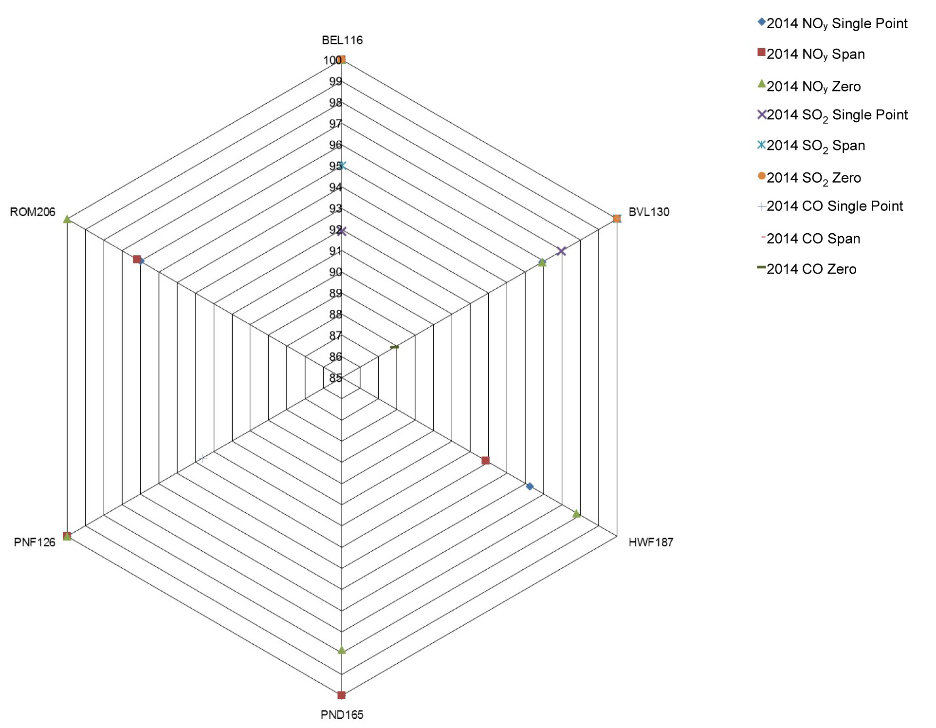
Figure 4-1 provides a map of the CASTNET continuous trace-level gas monitoring site locations. All sites were operated according to the CASTNET QAPP Appendix 11, Procuring, Installing, and Operating NCore Air Monitoring Equipment at CASTNET Sites (Amec Foster Wheeler, 2013). The CASTNET QAPP and all related appendices can be accessed on the EPA CASTNET website.
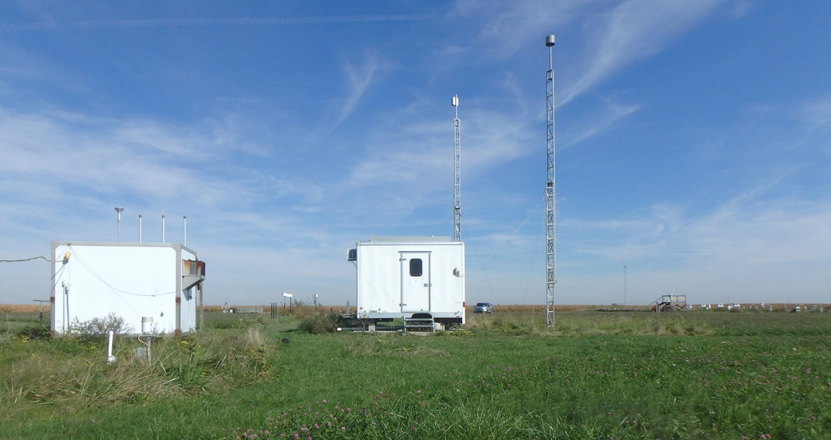
Bondville, IL (BVL130)
Quality Assurance Program Results
Continuous Trace-level Gas Concentrations
Continuous trace-level gas QC criteria are set forth in 40 CFR Part 58 Appendix A (EPA, 2013a) for NOy (including the criteria pollutant NO2), SO2, and CO. Figure 4-a presents summary statistics of critical criteria measurements at trace-level gas monitoring sites collected during 2014. All data associated with QC checks that fail to meet the established criteria were invalidated unless the cause of failure was documented to have no effect on ambient data collection. QC failures for EPAsponsored sites are addressed in quarterly QA reports, which can be found on the EPA CASTNET website.
Figures 4-2 and 4-3 present 2014 annual average hourly composite diurnal profiles of SO2, NOy, and O3 for BEL116 and BVL130, respectively. Figures 4-4 through 4-8 show the 2014 annual average hourly composite diurnal profiles of NOy and O3 for MAC426, HWF187, PNF126, PND165, and ROM206. Figure 4-9 shows the November through December 2014 average hourly profile for GRS420. The profiles in Figures 4-2 through 4-9 were constructed by averaging all values from the same hour for their respective time periods. Different scales were used for y-axes (SO2 and NOy) in the eight diagrams. The figures illustrate that differences in geography, terrain, and elevation affect the evolution of photochemically reactive pollutants in the boundary layer.
Table 4-2 Summary of 2014 Minimum and Maximum Values from Diurnal Charts
| Site Location* | Site Elevation (meters) | NOy(ppb) | O3(ppb) | ||
|---|---|---|---|---|---|
| Min | Max | Min | Max | ||
| BEL116, MD | 47 | 5.6 | 12.4 | 16 | 42 |
| BVL130, IL | 213 | 3.5 | 5.4 | 22 | 40 |
| MAC426, KY | 243 | 2.7 | 3.8 | 24 | 41 |
| HWF187, NY | 497 | 0.8 | 1.1 | 20 | 34 |
| GRS420, TN1 | 793 | 1.9 | 3.4 | 26 | 30 |
| PNF126, NC | 1,216 | 1.2 | 1.5 | 37 | 41 |
| PND165, WY | 2,386 | 0.7 | 1.0 | 43 | 49 |
| ROM206, CO | 2,742 | 0.7 | 1.4 | 46 | 53 |
Note:
* Sites are listed in order of elevation
1 November through December 2014, only
Continuous Trace-level NOy and Ozone
The minimum and maximum mean composite NOy and O3 concentrations shown in Figures 4-2 through 4-9 are summarized in Table 4-2. The sites are listed in order of elevation. The highest NOy concentrations were measured at BEL116, a suburban Maryland site with nearby high mobile-source NOx emissions. Low NOy values were recorded at the six rural sites in Kentucky, New York, Tennessee, North Carolina, Wyoming, and Colorado. The eight profiles in Figures 4-2 through 4-9 illustrate the loss of O3 during the late afternoon and nighttime hours and its production during daylight hours. The diurnal change was less pronounced at the six rural sites. The BEL116 site observed the largest nighttime loss and subsequent highest daytime production, an average increase of about 25 ppb of O3 for 2014. The BVL130 data illustrate a typical diurnal relationship between NOy and O3 concentrations with high NOy concentrations associated with vehicular NOx emissions in the morning and evening and elevated O3 concentrations in the afternoon. The data from MAC426 also show a diurnal evolution with the highest NOy concentrations in the morning and the evening and highest O3 concentrations in the afternoon. The MAC426 data appear similar to measurements made at an urban site.
O3 and NOy concentrations were also measured at HWF187, GRS420, PNF126, PND165, and ROM206 during 2014. Of these sites, the highest O3 concentration was measured at ROM206. The concentrations measured at the three sites with the highest elevations show less 24-hour variation than the other five sites because of the absence of nighttime O3 loss/depletion mechanisms near the high-elevation monitors (Talbot et al., 2005). Nighttime dry deposition is low because shallow boundary layers that affect sampler intakes (10 m for O3) typically do not form at these high-elevation sites, and scavenging is low because fresh nitric oxide is not available to react with O3 (Talbot et al., 2005). The ROM206 data suggest a large production or transport of NOy around sunset. There are no significant NOx sources in the immediate area. The increase in NOy is likely a result of the advection of polluted air masses from the Front Range Urban Corridor and the frequent late afternoon upslope flow from the east (Baumann et al., 1997).
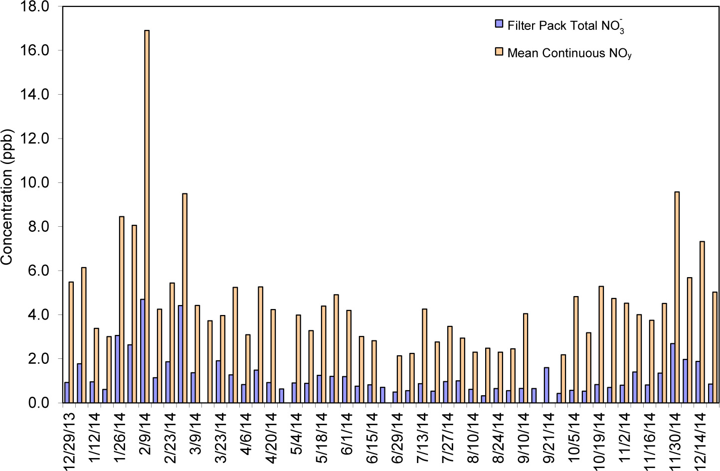
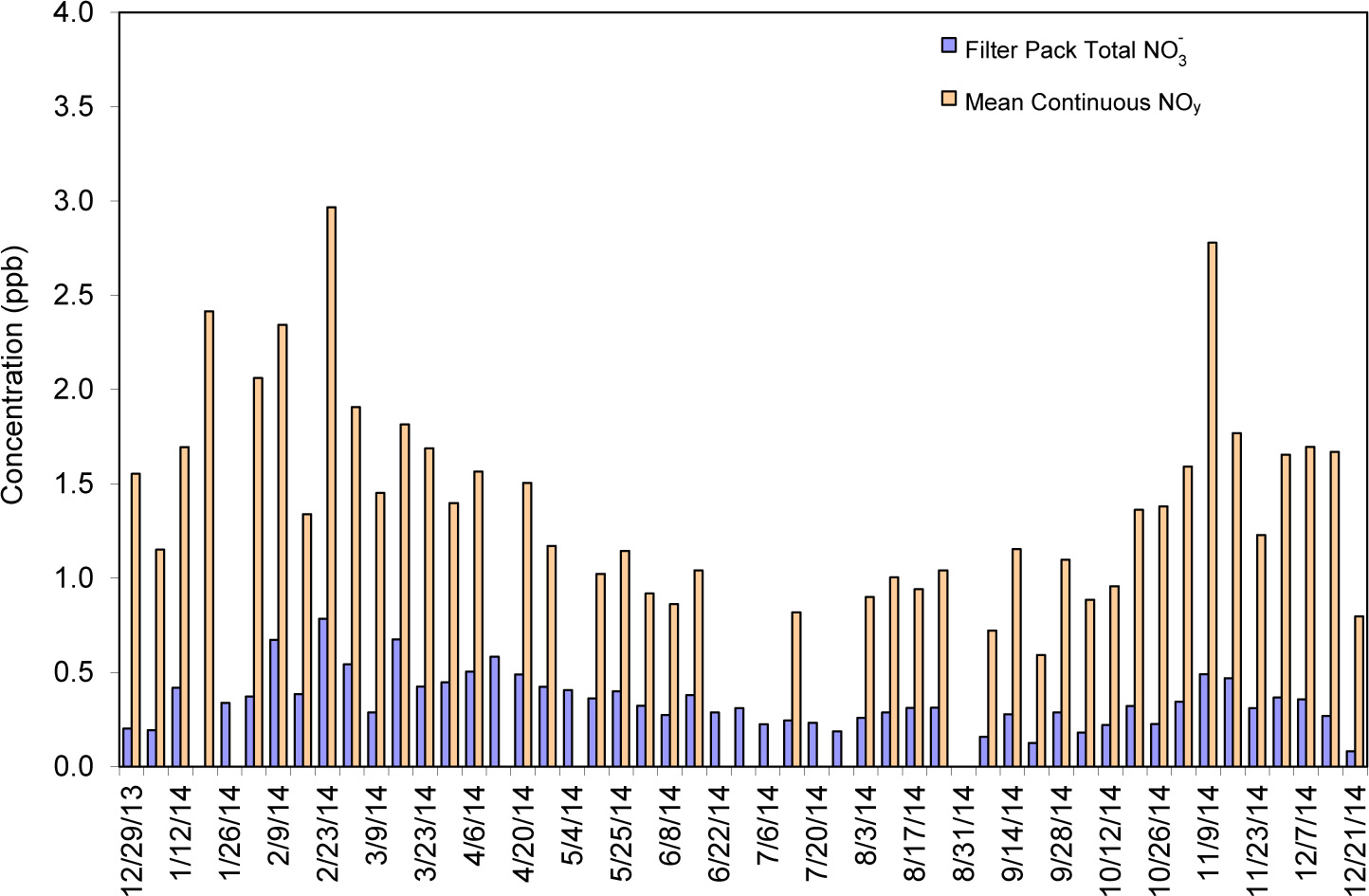
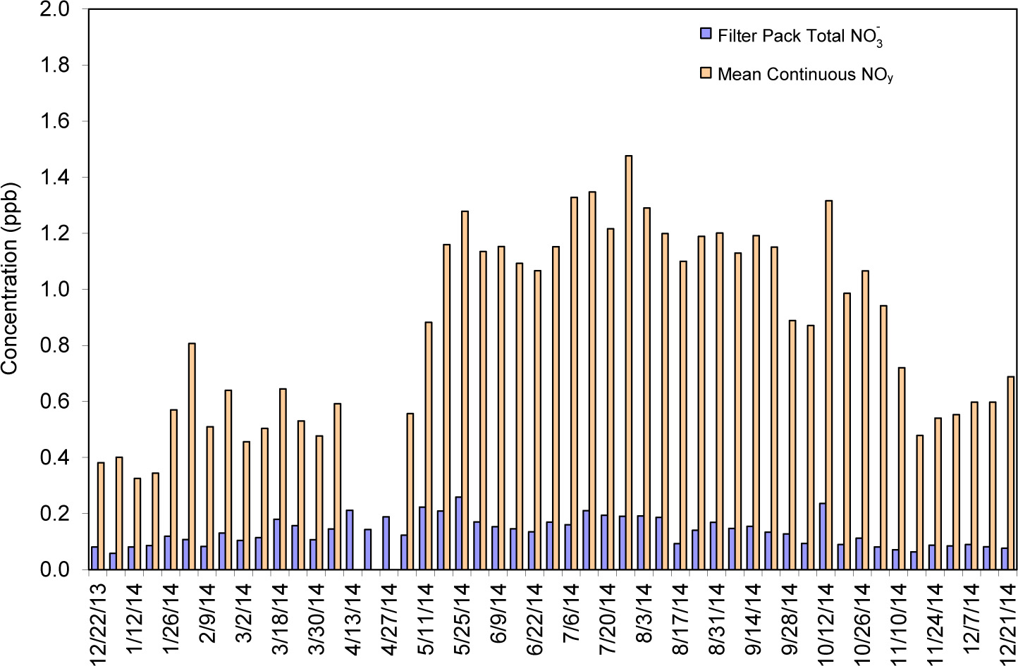
Continuous Trace-level NOy and Filter Pack Total Nitrate Concentrations
HNO3 and particulate NO3- are measured on CASTNET filter packs, and the sum is reported as total NO3-. Because HNO3 and particulate NO3- are measured as components of NOy, NOy concentrations should always be higher than total NO3- levels, i.e., the ratio of NOy to total NO- 3 should always be greater than 1.0. A comparison of weekly mean continuous NOy concentrations with filter pack total NO3- levels at BVL130, PNF126, and PND165 for 2014 was used to evaluate the measurements (Figures 4-10 through 4-12). The NOy concentrations were consistently higher than the total NO3- levels, as expected. The results are similar for the other five sites. Figure 4-12 shows relatively high NOy concentrations were measured at PND165 during the warm season, approximately May through September. The average of weekly filter pack total NO3- concentrations, the average weekly mean continuous NOy levels, and their ratios for the eight sites are listed in Table 4-3. These were calculated as the average of all valid weekly filter pack concentrations and the average of mean continuous NOy values matching the run time of the weekly filter packs. Average weekly mean NOy levels were higher than the average of weekly total NO3- concentrations with ratios of NOy to total NO- 3 varying from 4.17 at BVL130 to 10.04 at BEL116. The highest average of weekly concentrations (1.22 ppb) of total NO3- at BVL130 resulted in the lowest ratio of 4.17.
Table 4-3 Summary of the Average of Weekly Filter Pack Total NO3- and Weekly Mean Continuous NOy Measurements for 2014
| Site Location | Total NO3 (ppb) | NOy (ppb) | Ratio |
|---|---|---|---|
| BEL116, MD | 0.80 | 7.20 | 10.04 |
| BLV130, IL | 1.22 | 4.65 | 4.17 |
| MAC426, KY | 0.79 | 3.25 | 4.45 |
| HWF187, NY | 0.22 | 0.99 | 4.38 |
| GRS420, TN* | 0.54 | 2.61 | 6.69 |
| PNF126, NC | 0.35 | 1.41 | 4.21 |
| PND165, WY | 0.14 | 0.87 | 6.38 |
| ROM206, CO | 0.19 | 1.03 | 6.13 |
Note: * November through December 2014, only
Figure 4-10 Comparison of BVL130, IL Weekly Mean Continuous Trace-level NOy and Filter Pack Total NO3- Concentrations
 Download Image
Figure 4-11 Comparison of PNF126, NC Weekly Mean Continuous Trace-level NOy and Filter Pack Total NO3- Concentrations
 Download Image
Figure 4-12 Comparison of PND165, WY Weekly Mean Continuous Trace-level NOy and Filter Pack Total NO3- Concentrations
 Download Image
Continuous Trace-level and Filter Pack Sulfur Dioxide Concentrations
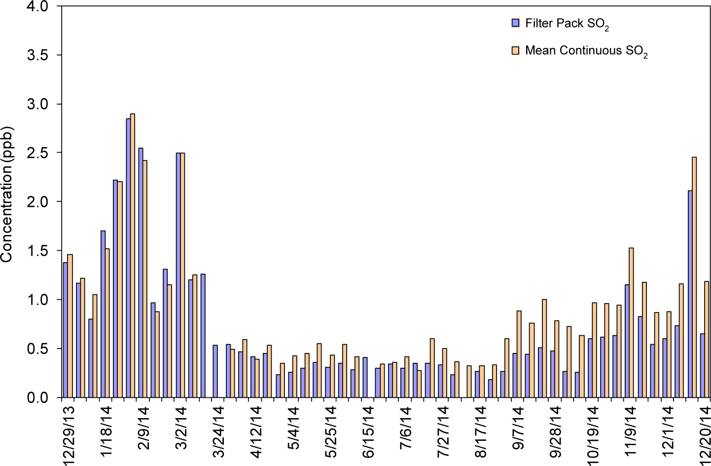
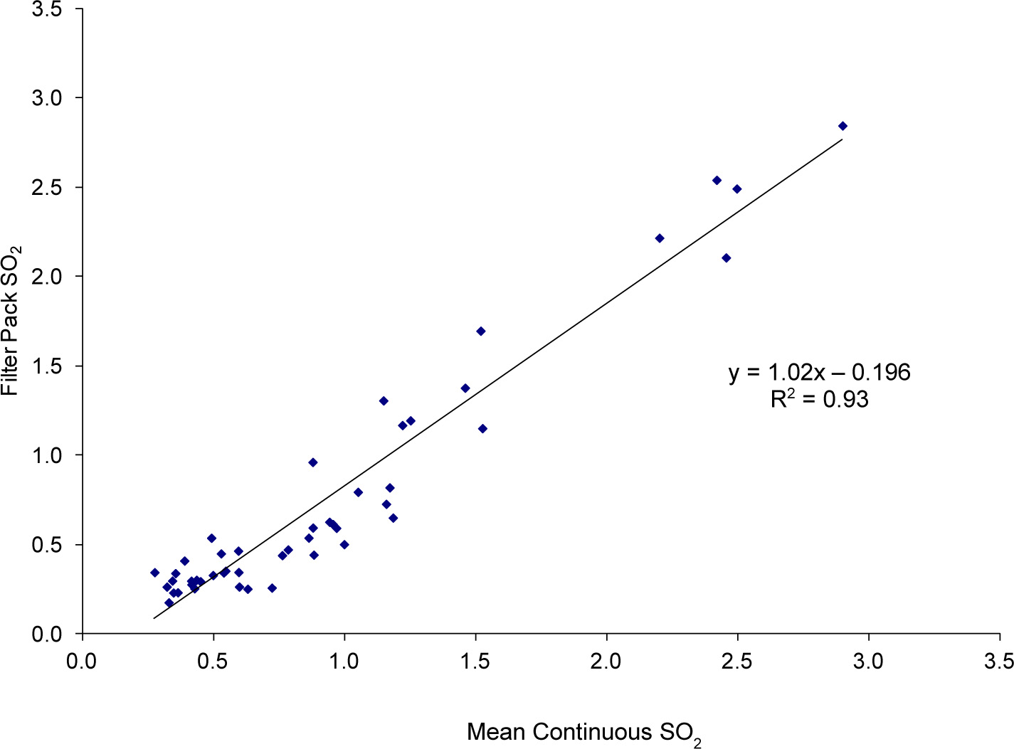
Hourly average continuous trace-level and weekly filter pack concentrations of SO2 were collected at the BEL116 and BVL130 sites during 2014. The comparison of trace-level continuous data with filter pack concentration data is performed routinely to evaluate both measurements. Figure 4-13 provides a bar chart that compares weekly aggregated SO2 data from the continuous analyzer with weekly integrated filter pack SO2 measurements at the BEL116 site. There was a positive relationship between the continuous analyzer and filter pack measurements with a regression line (Figure 4-14):
y = 1.02x – 0.196.
The correlation coefficient for the two sets of measurements is 0.93.
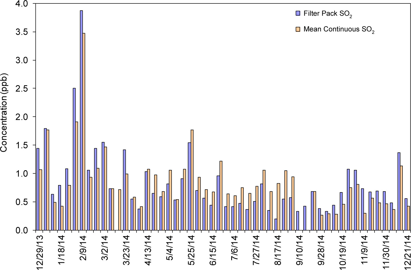
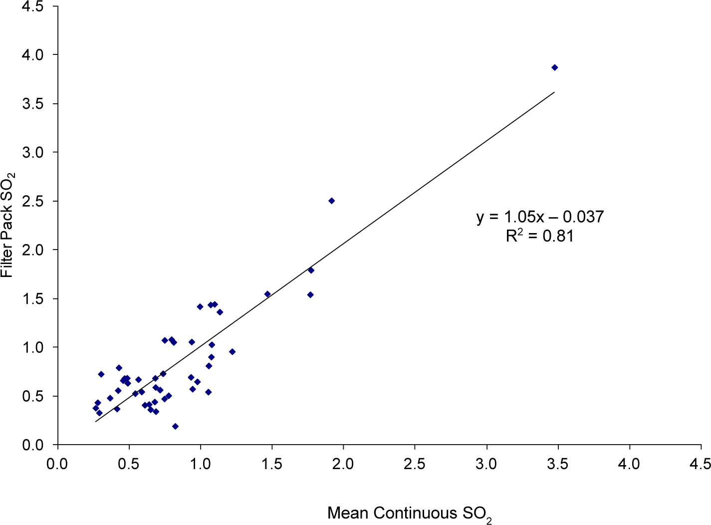
Figure 4-15 provides a bar chart for BVL130 that compares weekly mean SO2 data from the continuous analyzer with weekly filter pack SO2 measurements. The continuous and filter pack SO2 data for 2014 have a regression line (Figure 4-16):
y = 1.05x – 0.037.
The correlation coefficient for the two sets of measurements is 0.81.
Figure 4-13 Comparison of BEL116, MD Weekly Mean Continuous Trace-level and Filter Pack SO2 Concentrations
 Download Image
Figure 4-14 Scatter Plot of BEL116, MD Weekly Mean Continuous Trace-level and Filter Pack SO2 Concentrations (ppb) for 2014
 Download Image
Figure 4-15 Comparison of BVL130, IL Weekly Mean Continuous Trace-level and Filter Pack SO2 Concentrations
 Download Image
Figure 4-16 Scatter Plot of BVL130, IL Weekly Mean Continuous Trace-level and Filter Pack SO2 Concentrations (ppb) for 2014
 Download Image
Chapter 5: Update on the Ammonia Monitoring Network (AMoN)
AMoN utilizes passive ammonia samplers at a total of 92 locations, 65 of which are located at CASTNET sites. AMoN operates under the NADP. The network has been in operation since 2007 and provides information on 2-week integrated ammonia concentrations. The goal of AMoN is to grow the network to more than 300 sites covering all sensitive ecoregions of the continental United States.
Atmospheric gaseous NH3 concentrations have become more important in terms of air quality and atmospheric chemistry over the past 10 years. Measurements have shown that reactive NH3 concentrations and deposition fluxes have changed little despite significant reductions in NOx emissions nationwide (Puchalski et al., 2011). NH3 is the most prevalent base gas in the atmosphere and is released into the air from a variety of biological sources, as well as from industrial and combustion processes, with the largest sources of emissions in the agricultural sector, mostly from animal waste and commercial fertilizer application. Although NH3 has beneficial applications, such as increased agricultural production from NH3-based fertilizer use, it can also have a detrimental effect on the environment when it reacts with acidic ions such as SO42- and NO3- to form ammonium sulfate [(NH4)2SO4] and ammonium nitrate (NH4NO3) particles, which are significant components of PM2.5. NH3 and NH4+ particles also contribute to visibility degradation and the atmospheric deposition of nitrogen to sensitive ecosystems. Human health effects include short-term eye and lung irritation and long-term cardiovascular system impacts through inhalation of the fine particles.
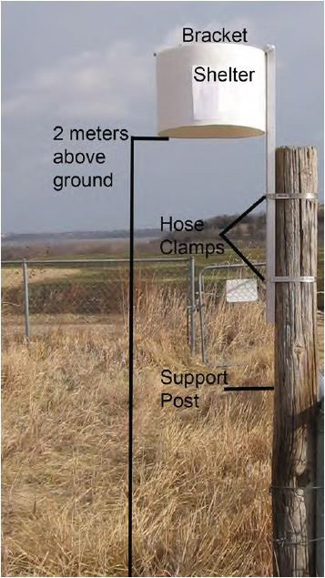
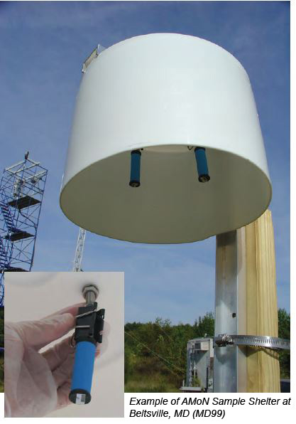
NADP/AMoN deploys Radiello samplers (Figure 5-1), which are easy to deploy and are costeffective. Sample preparation and extraction are straightforward. The samplers are deployed for 2-week periods and do not require electricity or a data logger for operation.
Beltsville, MD (BEL116)
Figure 5-1 Radiello Sampler
Source: NADP/AMoN (2015)
The objectives of AMoN are to:
- Assess long-term trends in ambient NH3 concentrations and depositions of reduced nitrogen species,
- Provide input data and evaluate atmospheric models,
- Provide better estimates of total nitrogen inputs to ecosystems,
- Assess changes in atmospheric chemistry associated with SO2 and NOx emission reductions,
- Assess compliance with PM2.5 standards, and
- Evaluate possible long-term climate effects related to spatial and temporal trends of NH3 gas in the atmosphere.
Source: NADP/AMoN (2015), AMoN Factsheet.
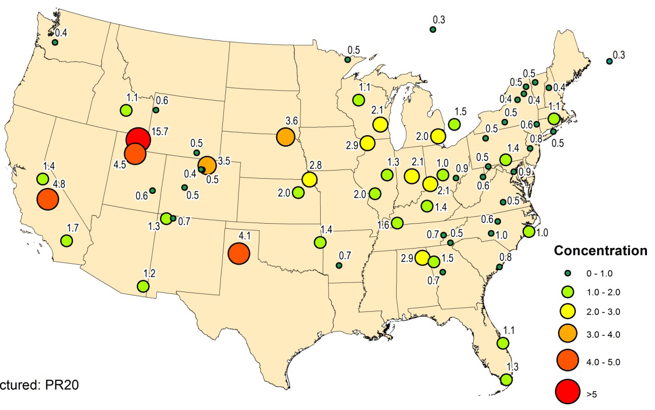
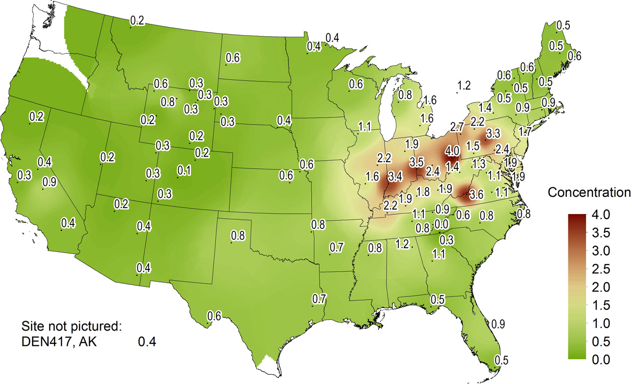
Annual mean NH3 concentrations for 2014 for the 66 sites that met completeness requirements are mapped in Figure 5-2 and show a wide range of concentrations from a low of 0.3 μg/m 3 in Canada at the Nova Scotia (NS01) and Ontario (ON25) sites to a high of 15.7 μg/m 3 in northern Utah (UT01). The Utah monitoring site is situated on a Utah State University research farm, and small quantities of livestock are often on the farm (Martin and Baasandorj, 2016). The site is located in a valley with frequent periods of stagnant weather. The next highest annual mean NH3 concentrations ranged from 3.5 to 4.8 μg/m 3 at five sites west of the Mississippi River. The highest concentration east of the Mississippi was observed at sites in northern Alabama (AL99) and northern Illinois (IL37) where each site measured a concentration of 2.9 μg/m 3. High local NH3 concentrations are largely influenced by agricultural operations (e.g., cattle feeding and waste and crop fertilization and production).
Ten AMoN sites have been operating since late 2007. However, because of data incompleteness, annual means for these sites could not be calculated prior to 2009 data. Table 5-1 presents 2009 and 2014 annual mean concentrations and the percent differences in concentrations from 2009 to 2014. All 10 sites measured higher concentrations in 2014 than 2009 and support the observation that reactive NH3 concentrations have increased or shown little change despite lower SO2 and NOx emissions, which in turn have resulted in lower atmospheric (NH4)2SO4 and NH4NO3 and perhaps higher NH3 concentrations. These results also support the continued need for an NH3 network since concentrations are likely increasing, at least in certain locations (Puchalski et al., 2011).
Table 5-1 Annual Mean NH3 Concentrations at 10 AMoN Sites
| Site ID* | 2009 | 2014 | Percent Changed | ||
|---|---|---|---|---|---|
| Concentration (μg/m 3) | N | Concentration (μg/m 3) | N | ||
| CO13 | 3.4 | 26 | 3.5 | 25 | +2 |
| IL11 | 1.1 | 25 | 1.3 | 26 | +16 |
| IN99 | 1.3 | 24 | 2.1 | 22 | +66 |
| MN18 | 0.3 | 26 | 0.5 | 26 | +75 |
| OH02 | 0.6 | 26 | 0.9 | 26 | +53 |
| OH27 | 1.4 | 27 | 2.1 | 26 | +49 |
| OK99 | 1.2 | 26 | 1.4 | 26 | +19 |
| SC05 | 0.3 | 26 | 0.8 | 23 | +200 |
| TX43 | 2.9 | 27 | 4.1 | 27 | +42 |
| WI07 | 1.9 | 26 | 2.1 | 26 | +14 |
Note:
*AMoN site information can be found at http://nadp.sws.uiuc.edu/amon/. By convention, the first two alphabetic characters of the NADP site identification are the state abbreviation where the site is located.
N = number of samples
Because the largest source of NH3 emissions is the agricultural sector, reactive NH3 concentrations and depositions are not related to the downward trend in sulfur and other nitrogen species (Amec Foster Wheeler, 2015a), which are more closely tied to power and industrial sector emissions and track relatively well with the emission reductions mandated by the CAAA. Also, NH3 emissions are released typically from area sources while power and industrial emissions are released from elevated point sources. Atmospheric NH3 concentrations and depositions are more complex because NH3 deposition is bidirectional; NH3 can be emitted from vegetation and soils and deposited from the atmosphere. AMoN results are used to support the NADP Total Deposition Science Committee total deposition maps and fill gaps in the reduced nitrogen budget across the United States.
In order to continue improving our understanding of the role of NH3 in air chemistry, ambient air quality and deposition, and their resultant impacts, both ecological and human health-related, NADP plans to grow the network to more than 300 sites across the United States. Additionally, new sites will generate additional data for regional model input and for evaluation of air quality and deposition models.
Chapter 6: Speciated Reactive Nitrogen Measurements
CASTNET currently measures NO/NOy at six EPA-sponsored sites and two NPS-sponsored sites using traditional chemiluminescence analyzers. While the data measured at the NOy sites are useful for analyzing total reactive oxidized nitrogen concentrations, one of CASTNET’s goals is to provide estimates of dry and total nitrogen deposition, which is problematic without further speciation of the NOy measurements. Deposition velocities can vary significantly among the oxidized nitrogen species composing NOy, and uncertainties in deposition velocity of individual species leads to uncertainties in deposition calculations. Amec Foster Wheeler previously operated a NO/NOx/NOy analyzer at the Beaufort, NC (BFT142) CASTNET site (Baumgardner et al., 2014), which provided estimates of NO2 and NOz. The monitoring system utilized two molybdenum converters. The results showed that, at times, NOx concentrations were higher than NOy concentrations indicating an overestimation of NOx. In 2014, an enhanced analyzer with additional converters was installed at the BEL116, MD site to better estimate speciated nitrogen. The results from the BEL116 enhanced NOy analyzer are summarized in this chapter.
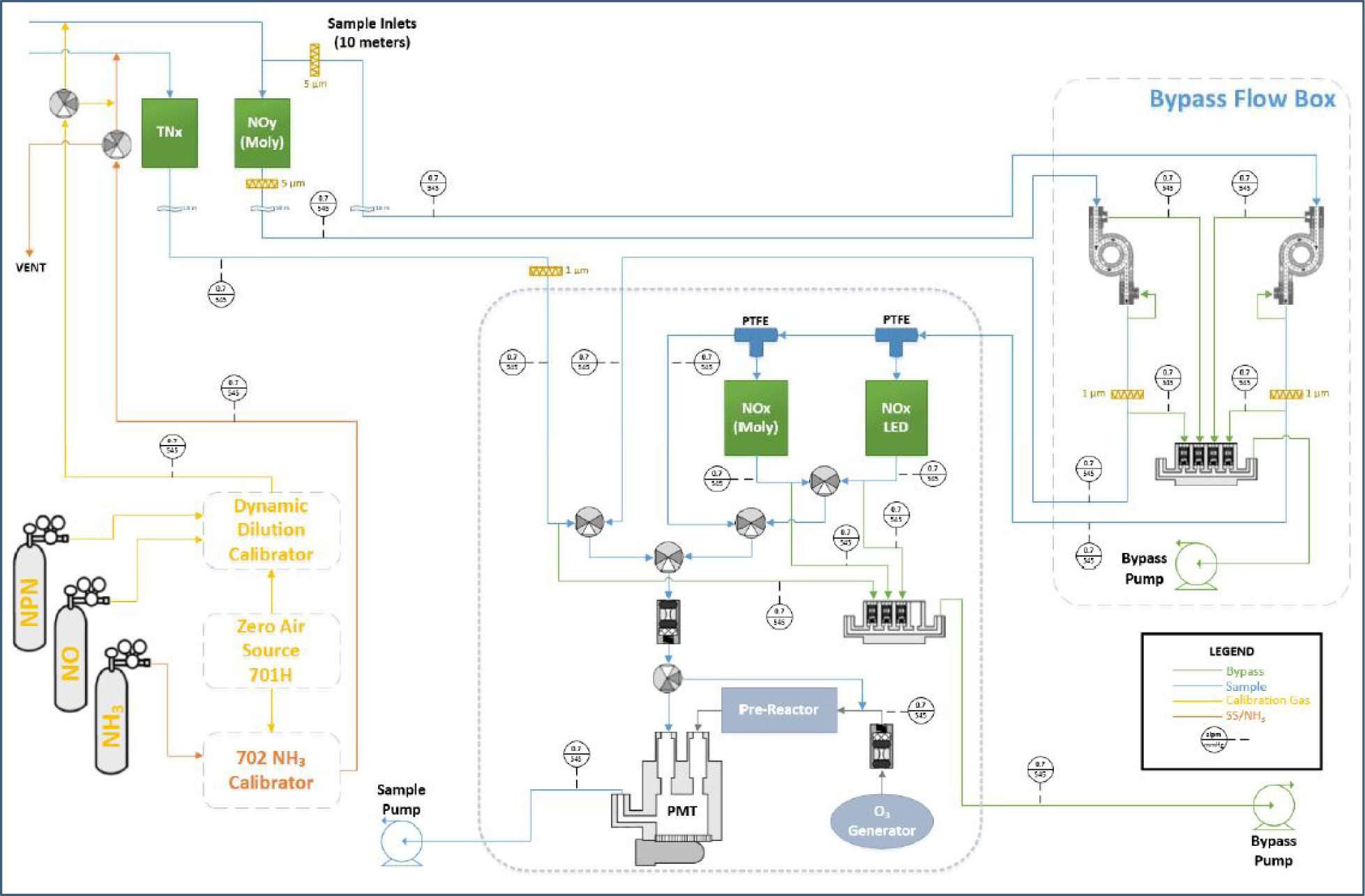
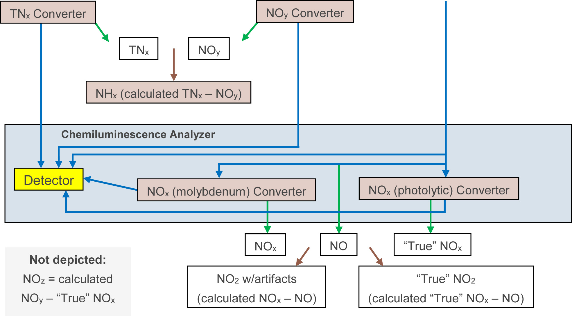
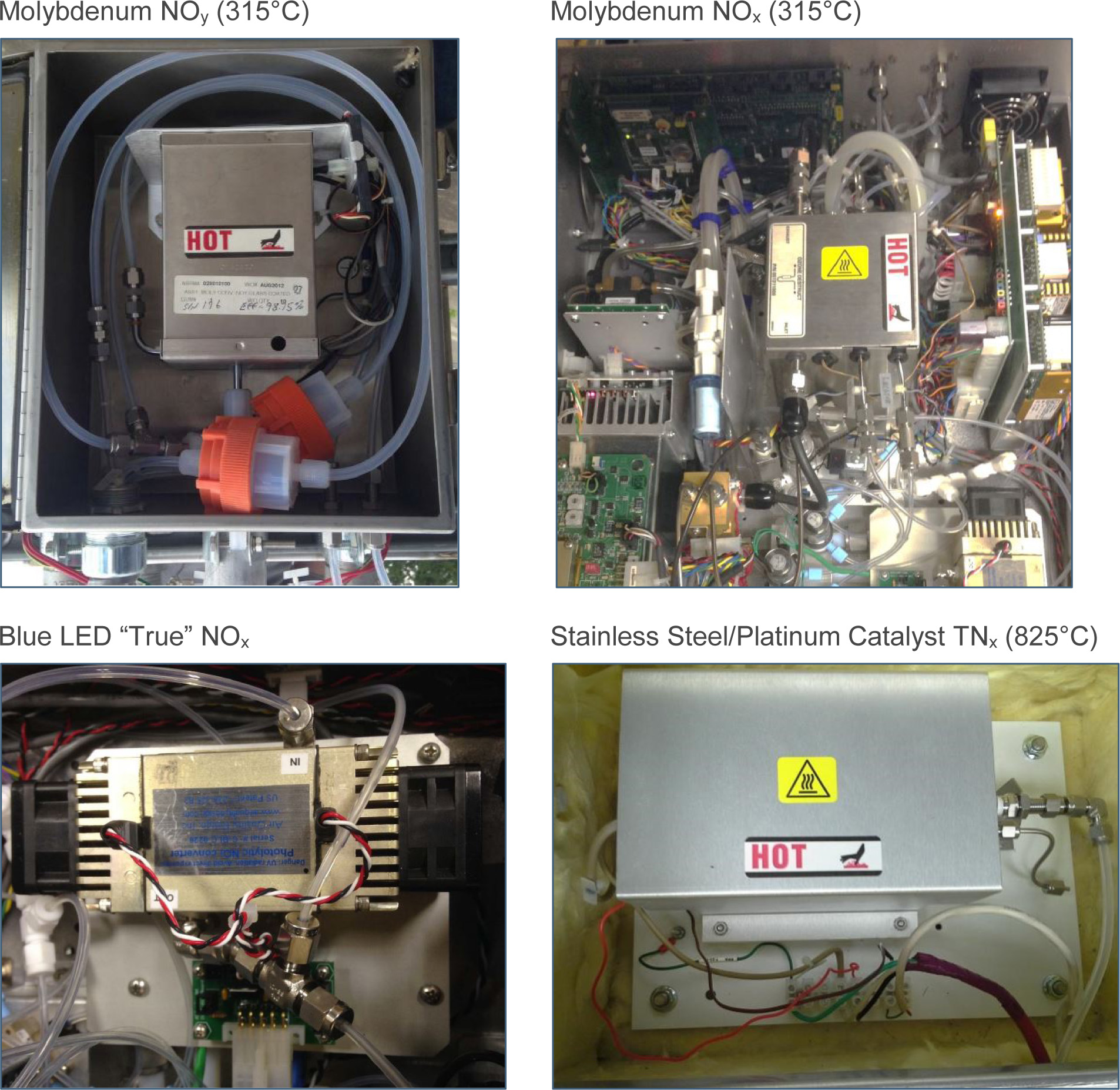
The goal of the enhanced NOy system study is to use a traditional NO detector to improve the speciated nitrogen measurements currently taken with the existing NO/NOy analyzers deployed at the eight CASTNET sites (see Chapter 4, Figure 4-1). NOx is measured using both a heated molybdenum converter and a light-emitting diode (LED) converter to evaluate any differences that occur using the molybdenum method. A stainless steel converter mounted on a 10-meter tower captures TNx, which is the total of NOy plus reduced reactive nitrogen, i.e., TNx = NOy + NHx, where NHx = NH3 gas + NH4+ aerosol. Inlet and absorption losses of HNO3 and NH3 are minimized by placing the converters near the inlet at 10 meters. By incorporating additional converters to a trace-level chemiluminescent NOy analyzer, the enhanced NOy monitor is designed to measure continuous concentrations of TNx, NOy, NOx, and NO, and, by difference, calculated concentrations of NHx, NOz, and NO2. A schematic of the enhanced NOy system is shown in Figure 6-1. A flow chart of the enhanced NOy system is shown in Figure 6-2. The converters used in the enhanced NOy measurement system are shown in Figure 6-3.
Deposition velocities vary significantly among nitrogen species. Detailed information on concentrations of specific species will improve nitrogen deposition estimates.
The enhanced NOy system was deployed at the BEL116, MD site in November 2014. The measurements from the enhanced system were compared with measurements from the other nitrogen monitoring systems at the BEL116 site, which included the Monitor for Aerosols and Gases in Ambient Air (MARGA) system, AMoN NH3 measurements, and the onsite CASTNET filter pack data. The measurement period used for the comparison was November 2014 through June 2015.
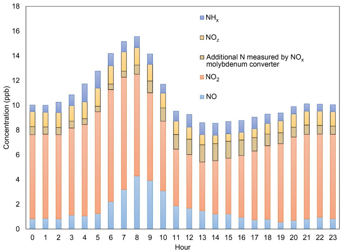
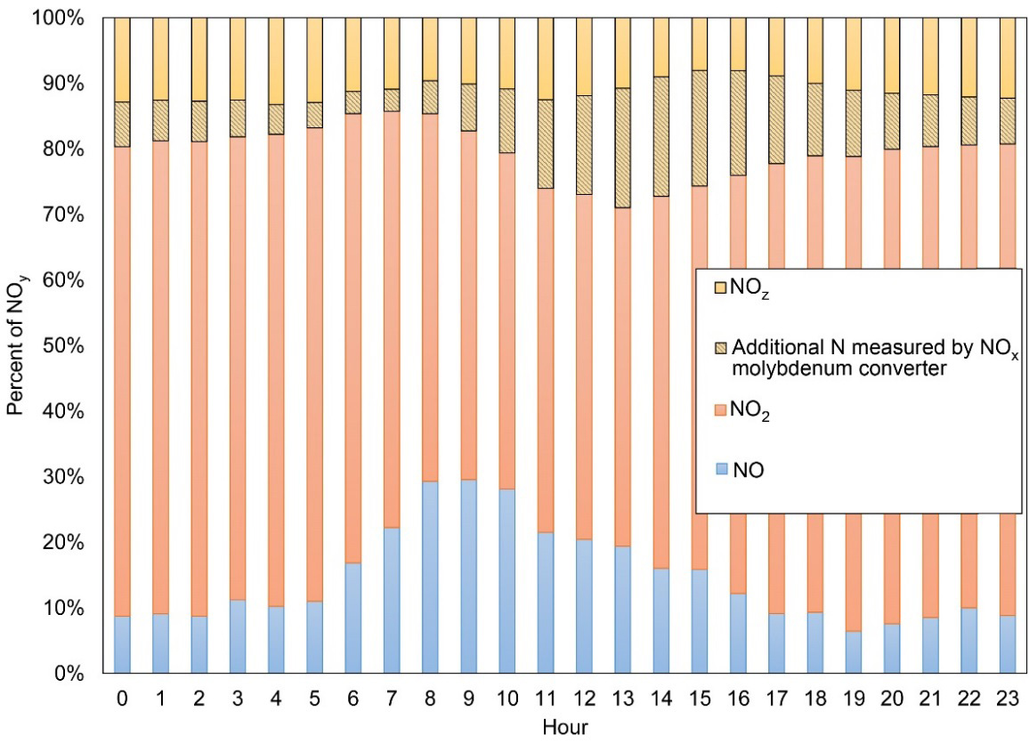
Measurements taken using the speciated nitrogen system over the 8-month measurement period are summarized in Figures 6-4 through 6-9. Figure 6-4 shows a diurnal concentration profile aggregated over the 8-month measurement period. It illustrates the build-up of NO in the morning from fresh vehicular emissions. All nitrogen species increased during the morning and then declined in the late morning and early afternoon. Figure 6-5 illustrates the diurnal percentages of NO, NO2, additional nitrogen (N) measured by the NOx molybdenum converter, and NOz aggregated over the monitoring period. The percentage of NO increased during the morning and eventually declined throughout the day. Based on nitrogen measurements made at the Beaufort, NC (BFT142) CASTNET site, NOx measurements overestimate actual concentrations as shown by the additional N measured by the NOx molybdenum converter (Baumgardner et al., 2014).
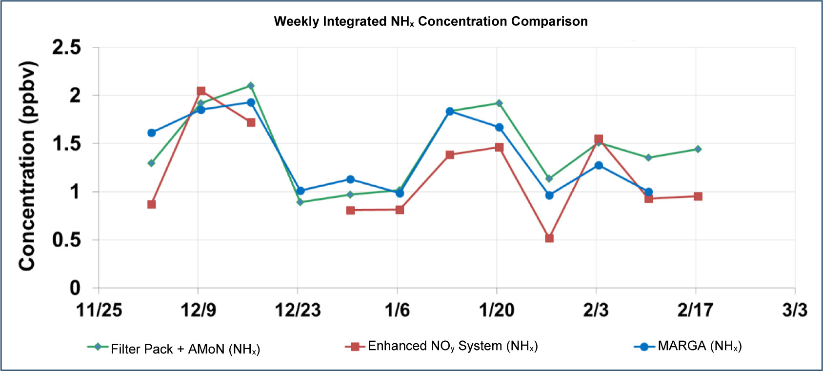
Figure 6-6 compares the enhanced NOy system and MARGA measurements with AMoN NH3 plus filter pack NH4+ data, which, when summed (NH3 + NH4+ ), give NHx values. The figure shows that the three sets of measurements follow similar temporal distributions, but the AMoN + filter pack estimates of NHx were 30 to 40 percent higher than the NHx measured by the enhanced NOy system (Mishoe et al., 2015). The difference was equivalent to the amount of NHx not accounted for by the enhanced NOy system due to the conversion of NHx by the molybdenum converter in addition to the NOy it was designed to convert.
Figure 6-7 depicts test results demonstrating the conversion of NHx in the molybdenum converter. The test was performed by streaming NH3 at 90 ppb into the converter and varying the temperature of the converter. The 90 ppb NH3, which was introduced at 12:20 local time, was streamed during the entire test period. Figure 6-7 shows that 90 ppb NH3 would read as 23 ppb NOy at 315°C. This result translates to an approximate 25 percent conversion that the system will read as additional NOy. The graph in Figure 6-7 is an example of the results of one of nine converters that were tested. The other tests not shown demonstrate about a 25 to 30 percent conversion.
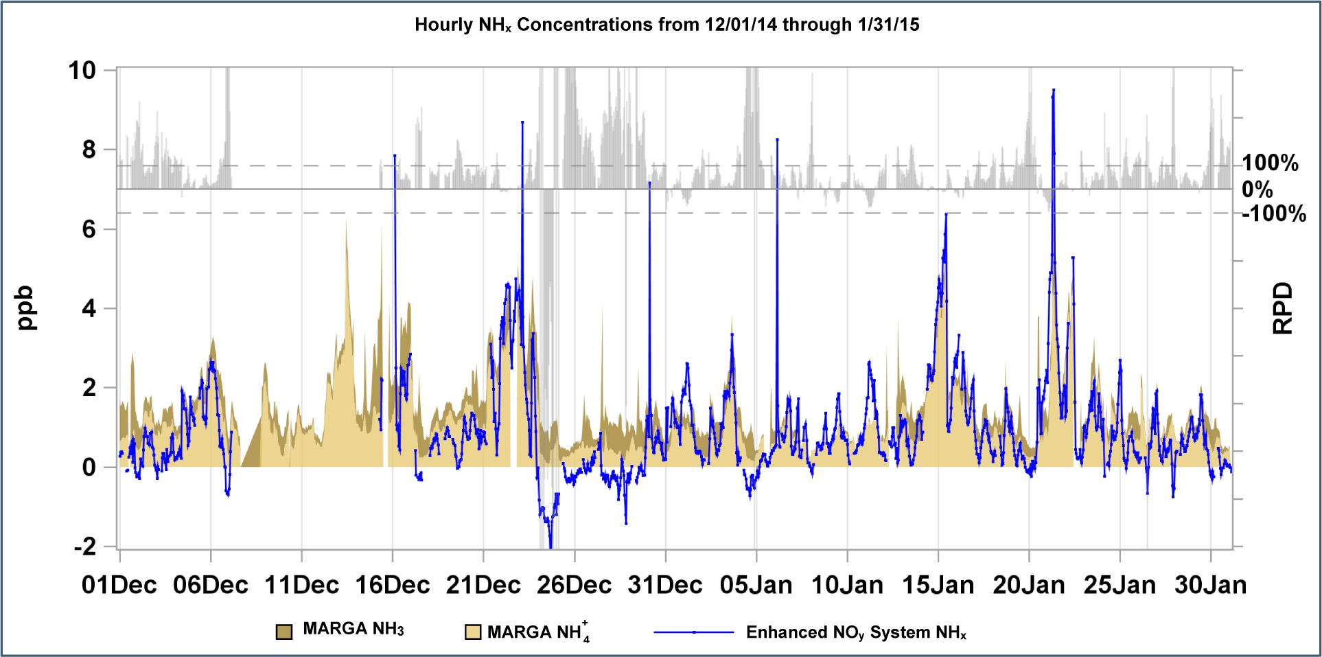
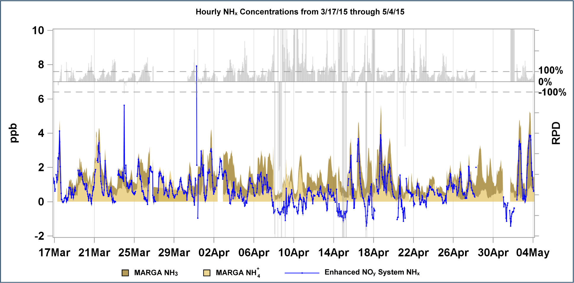
Figures 6-8 and 6-9 provide a comparison of the enhanced NOy system NHx (blue line), MARGA NH3 (dark), and MARGA NH4+ (light) measurements and the relative percent differences (RPD) between the enhanced the NOy system and the MARGA NHx measurements. The MARGA measurements were higher most of the time. Mishoe et al., (2015) discusses the overconversion in the NOy channel that biases the calculation for the enhanced NOy system data. The spikes were caused by desorption of the calibration gas from instrument tubing. Development of reporting limits for the enhanced NOy system data are underway in order to eliminate the negative values.
Again, deposition velocities vary significantly among the nitrogen species, and detailed information on specific species concentrations will improve nitrogen deposition estimates. To further this goal, the addition of a HNO3 channel to the enhanced analyzer might be implemented in future studies. By adding a second NOy channel and a scrubbing denuder, hourly HNO3 concentrations could be calculated by difference.
Figure 6-4 Composite Diurnal Variation of Components of Total Nitrogen from BEL116 for November 2014 through June 2015
 Download Figure
Figure 6-5 Composite Diurnal Variation of Components of NOy by Percentage from BEL116 for November 2014 through June 2015
 Download Figure
Figure 6-6 Time Series of Weekly NHx Concentrations for November 2014 through February 2015
 Download Figure
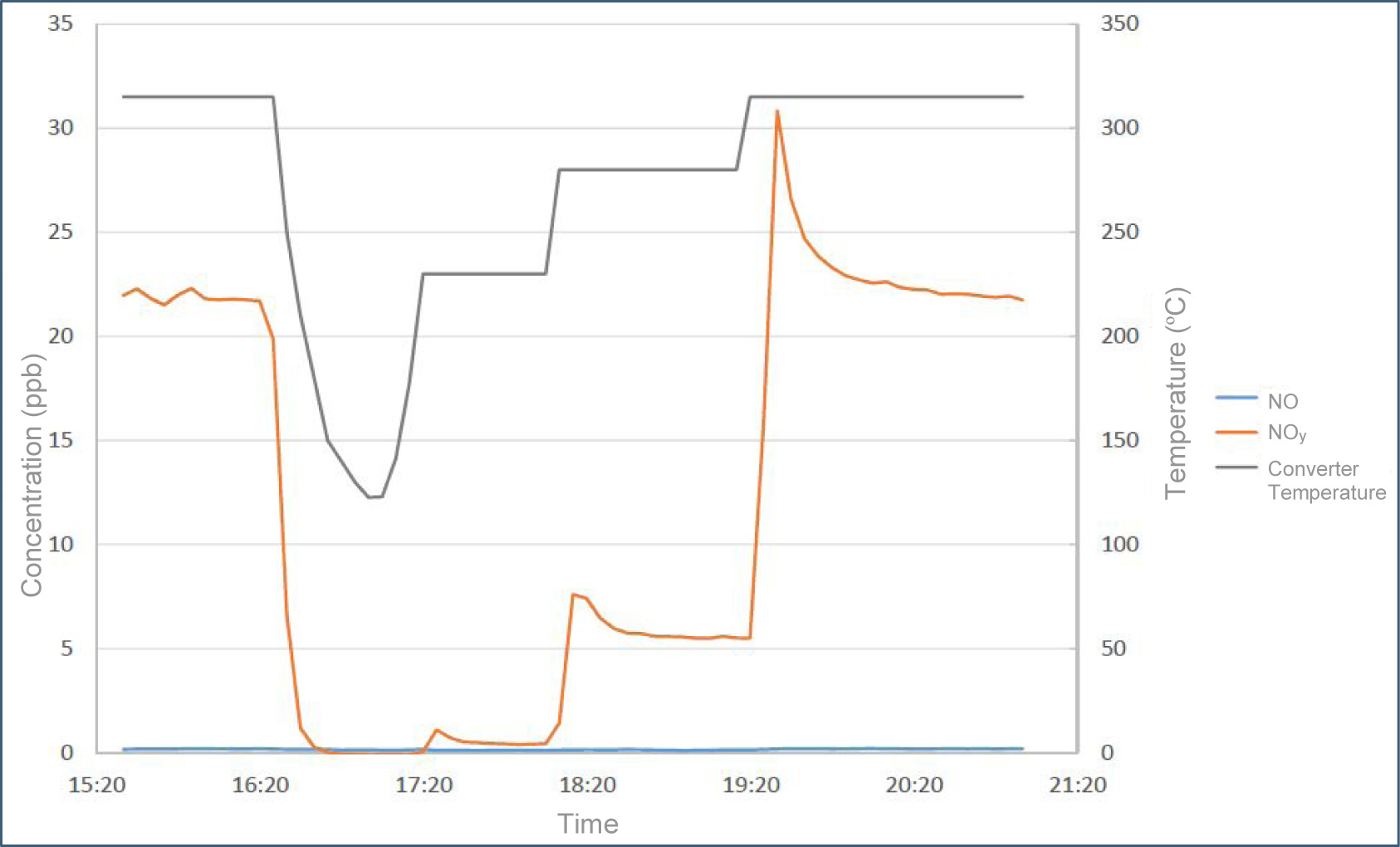
Figure 6-8 Enhanced NOy System and MARGA Measurements for December 2014 through January 2015 with Relative Percent Differences
 Download Figure
Figure 6-9 Enhanced NOy System and MARGA Measurements for March through May 2015 with Relative Percent Differences
 Download Figure
Chapter 7: Sulfur Pollutant Concentrations
Weekly average concentrations of sulfur dioxide and particulate sulfate were measured using 3-stage filter packs at 93 CASTNET monitoring stations during 2014. Trends in mean annual sulfur dioxide and sulfate concentrations were aggregated over 34 eastern and 16 western reference sites and are shown using box plots. Sulfur dioxide measured at the 34 eastern reference sites declined by 82 percent over the 25-year period from 1990 through 2014. Measured annual mean concentrations of sulfur dioxide and sulfate have decreased steadily since 2005. Sulfur dioxide and sulfate concentrations measured at the 16 western reference sites have decreased over the last 19 years, 1996 through 2014.
Maps of annual mean concentrations of SO2 and SO42- measured in 2014 are presented in this chapter. Additional maps of 2014 quarterly mean concentrations are provided in CASTNET quarterly data reports (Amec Foster Wheeler, 2014a; 2014b; 2015b; 2015c). Trends in annual mean concentrations over the 25-year period (1990 through 2014) were derived from measurements from the 34 CASTNET eastern reference sites and for the period 1996 through 2014 from data measured at 16 CASTNET western reference sites. See Appendix A for the designated reference sites.
Sufur Dioxide Concentrations
Annual mean SO2 concentrations are shown in Figure 7-1 for 2014. Annual mean concentrations were highest in the Midwest near the Ohio River.
Box plots of annual mean SO2 concentrations aggregated over the 34 eastern reference sites from 1990 through 2014 (right side) and the 16 western reference sites from 1996 through 2014 (left side) are depicted in Figure 7-2. The y-axes on the western and eastern plots have different scales because concentrations measured at the western CASTNET sites were much lower than those measured at the eastern sites. Three-year mean concentrations for the eastern reference sites for 1990–1992 and 2012–2014 were 8.8 μg/m 3 and 1.5 μg/m 3, respectively. This change constitutes an 82 percent reduction in 3-year mean SO2 concentrations between the two periods. The 2014 mean level of 1.6 μg/m 3 was slightly higher than the 2013 mean value of 1.4 μg/m 3 , which was the lowest concentration measured by the eastern reference sites in the history of the network and represents a significant decline from the 2005 concentration of 6.0 μg/m 3 . The higher 2014 concentration was caused by the higher SO2 emissions associated with the extreme cold during the first quarter of the year (see Chapter 8).
The box plots for the western reference sites indicate a decline in annual mean SO2 concentrations aggregated over the 16 sites. Three-year mean SO2 concentrations for 1996–1998 and 2012–2014 were 0.6 μg/m 3 and 0.3 μg/m 3 , respectively. This change constitutes a 50 percent reduction in 3-year mean SO2 concentrations at the CASTNET western reference sites over the 19 years.
The 2014 average sulfur dioxide concentration for the eastern reference sites was 1.6 μg/m 3. The eastern sulfur dioxide data show a substantive decline since 1997. The reduction (82 percent) in sulfur dioxide concentrations is consistent with the reduction (80 percent) in sulfur dioxide emissions from EGUs operating in the eastern United States, suggesting an approximately linear relationship between concentrations and emissions.
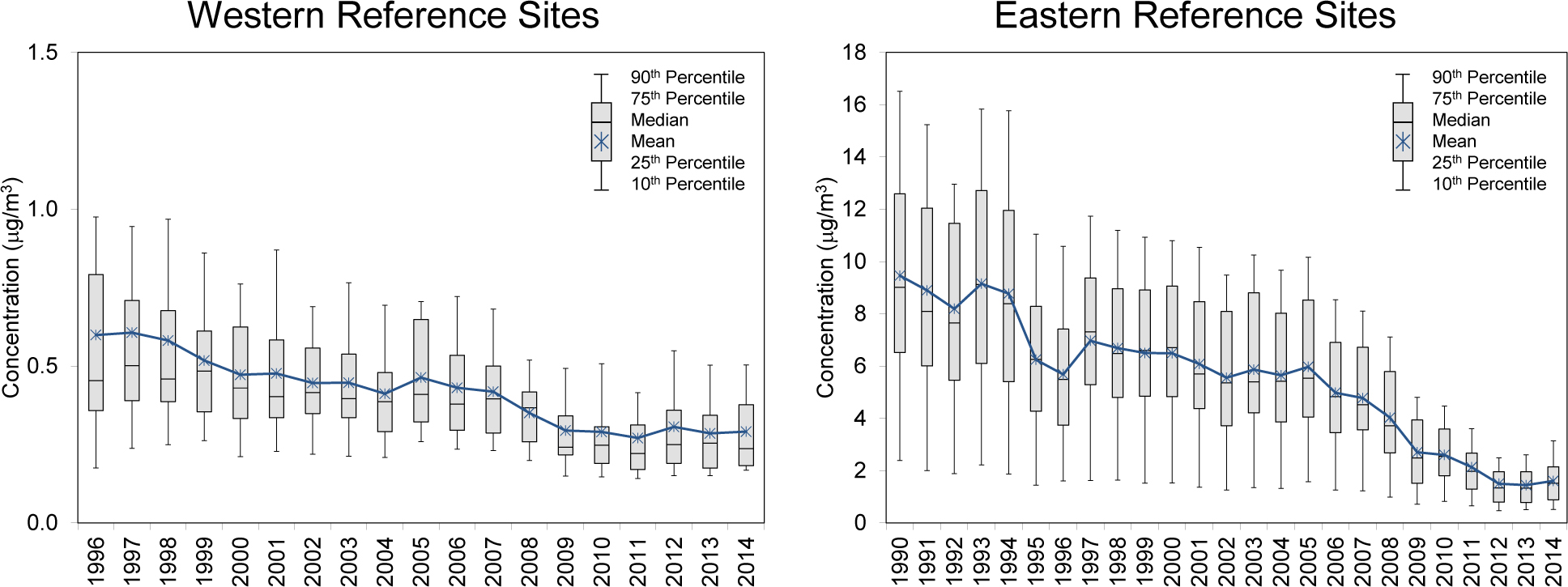
Figure 7-3 Trend in Annual Composite SO2 Emissions from Regulated EGUs Operating in Illinois, Indiana, Kentucky, Ohio, Pennsylvania, and West Virginia
 Download Figure
Figure 7-3 illustrates the trend in SO2 emissions from regulated EGUs from 1990 through 2014 aggregated over six states in the eastern United States. The 25-year decline in aggregated emissions was 80 percent, which is consistent with the 82 percent reduction (Figure 7-2) in annual mean SO2 concentrations aggregated over the CASTNET eastern reference sites.
Particulate Sulfate Concentrations
Figure 7-4 shows a map of 2014 annual mean particulate SO42- concentrations. Figure 7-5 provides box plots of annual mean SO42- concentrations from the 34 eastern reference sites and 16 western reference sites. The right side shows the trend in measurements from the eastern reference sites. The figure shows a substantial decline in SO42- over the 25 years. Of particular note, concentrations declined rapidly from 2005 through 2014. The difference between 3-year means from 1990–1992 to 2012–2014 represents a 63 percent reduction in SO42- from 5.4 μg/m 3 to 2.0 μg/m 3 , respectively. The 2014 mean SO42- level of 1.9 μg/m 3 was the lowest in the history of the network.
The box plots for the western reference sites are provided on the left side of Figure 7-5. The data show a 22 percent reduction in annual mean SO42- concentrations aggregated over the 16 sites with 1996–1998 and 2012–2014 concentrations of 0.8 μg/m 3 and 0.6 μg/m 3 , respectively.
The 2014 average sulfate concentration for the eastern reference sites was 1.9 μg/m 3 , the lowest level in the history of the network. The eastern sulfate data show a substantive decline since 1998. Sulfate concentrations declined more slowly than sulfur dioxide concentrations at the eastern reference sites. Western sulfate concentrations were lower and decreased at a slower rate than concentrations measured at the eastern sites.
Chapter 8: Polar Vortices during 2013–2014 Winter
The polar vortex, one of several semi-permanent weather systems of the earth, is an area of low pressure in the upper atmosphere that typically centers over two areas in the Northern Hemisphere: near Baffin Island, Canada and northeast Siberia. The vortex is strongest in the winter due to an increased temperature contrast between the polar regions and the mid-latitudes. On occasion, the polar vortex can be forced south of its usual position and/or a significant segment of the larger vortex system can break off and move southward. The southerly movement of a polar vortex typically results in below normal temperatures in the United States and increased demand for electricity. The associated high sulfur dioxide emissions produce higher than normal sulfur dioxide concentrations. However, the cold dry air resulting from a polar vortex intrusion inhibits the formation of particulate sulfate concentrations.
The polar vortex is a high altitude, low-pressure system that persists over the Arctic in winter (Kennedy, 2014). The right side of Figure 8-1 shows a strong phase of the polar vortex in mid- November 2013. Dark purple depicts the most frigid air tightly contained in an oval-shaped formation inside the invisible bowl. The light purple line forming the outermost boundary of the cold Arctic air is the jet stream in its normal west-to-east pattern.
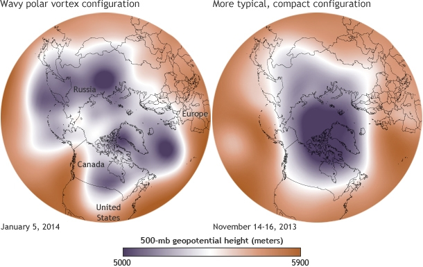
The first significant southerly intrusion of the polar vortex during the winter of 2013–2014 started in early December 2013. The jet stream pushed polar air southward causing record low temperatures and snow across the eastern United States over the period December 6–10, 2013 (Sosnowski, 2014). Approximately 100 daily snowfall records were broken across the northeastern, southeastern, and south central United States (National Centers for Environmental Information, 2013; 2014).
The second episode began in early January 2014 when the polar vortex weakened and broke apart, allowing fragments of cold air to move into the mid-latitudes. The image on the left side of Figure 8-1 shows the weakened vortex formation on January 5, 2014. The high pressure buildup in the Arctic caused the jet stream to slow down and flow farther south than usual, resulting in the advection of cold Arctic air into the central and eastern United States. This cold air advection produced significantly strong winds and bitter wind chills. During the week of January 7, 2014, at least 49 record daily lows were set across the United States (Rice, 2014).
Polar vortices were observed at other times in the eastern and south central United States during first quarter 2014. These meteorological events led to below normal temperatures and increased demand for electricity (North American Electric Reliability Corporation, 2014). Higher SO2 emissions and concentrations were measured during these events. Table 8-1 lists first quarter SO2 emissions and first quarter average SO2 concentrations for 11 states located in the upper Midwest and eastern/mid-Atlantic regions for 2012, 2013, and 2014.
The SO2 concentrations listed for each of the 11 states in Table 8-1 represent the average of all first quarter concentrations measured at the CASTNET sites in that state. Concentrations during first quarter 2014 were significantly higher than the previous two years. For example, quarterly mean concentrations measured at CASTNET stations in Indiana, Ohio, and Pennsylvania averaged 5.6 μg/m 3 for first quarter 2014 compared with a mean value of 3.3 μg/m 3 in first quarter 2013 and 3.1 μg/m 3 in first quarter 2012. The significantly higher state averages are attributed to the below-normal temperatures and associated higher fossil fuel use and emissions (Table 8-1). The 11-state average quarterly SO2 concentrations for 2014 were higher by 50 percent than the 2013 average and by 65 percent over the 2012 average.
SO2 emissions for first quarter 2012, 2013, and 2014 for these 11 states are also shown in Table 8-1. Major SO2 emissions sources are located in the upper Midwest and eastern/Mid- Atlantic regions. The average quarterly SO2 emissions for the 11 states in Table 8-1 for 2014 were higher by 20 percent with respect to the 2013 average and were higher by 28 percent than the 2012 average emissions.
Table 8-1 First Quarter 2012, 2013, and 2014 SO2 Emissions and Mean SO2 Concentrations
| State | 2012 | 2013 | 2014 | |||
|---|---|---|---|---|---|---|
| Emissions
(short tons) |
Concentration (μg/m 3) | Emissions
(short tons) |
Concentration (μg/m 3) | Emissions
(short tons) |
Concentration (μg/m 3) | |
| Illinois | 38,169 | 1.9 | 35,508 | 1.8 | 32,983 | 2.8 |
| Indiana | 64,048 | 2.6 | 74,084 | 2.8 | 91,215 | 4.9 |
| Kentucky | 44,782 | 2.1 | 52,602 | 2.6 | 54,698 | 3.5 |
| Michigan | 43,509 | 1.6 | 46,953 | 1.5 | 47,050 | 2.5 |
| New York | 3,494 | 1.1 | 6,539 | 1.1 | 10,558 | 1.9 |
| North Carolina | 11,777 | 0.8 | 11,306 | 0.9 | 11,557 | 1.1 |
| Ohio | 80,447 | 4.0 | 76,403 | 4.0 | 101,326 | 6.3 |
| Pennsylvania | 60,319 | 2.9 | 60,676 | 3.1 | 83,923 | 5.5 |
| Tennessee | 13,748 | 0.9 | 13,770 | 1.3 | 13,675 | 1.7 |
| Virginia | 7,091 | 2.3 | 10,903 | 2.5 | 14,415 | 3.1 |
| West Virginia | 16,092 | 1.7 | 19,795 | 2.1 | 28,602 | 3.2 |
| Total | 383,474 | -- | 408,537 | -- | 490,003 | -- |
| Average | 34,861 | 2.0 | 37,140 | 2.2 | 44,546 | 3.3 |
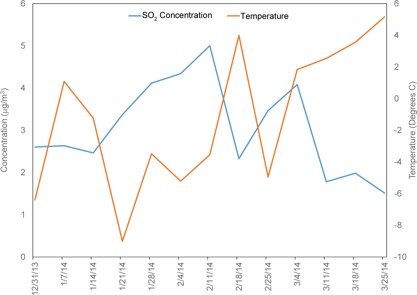
Figure 8-2 shows weekly SO2 concentrations and temperatures aggregated for the 34 CASTNET eastern reference sites. The graph shows a generally negative correlation between SO2 concentrations and ambient temperatures in that, as temperatures decrease, SO2 concentrations increase, and, as temperatures increase, SO2 concentrations decrease.
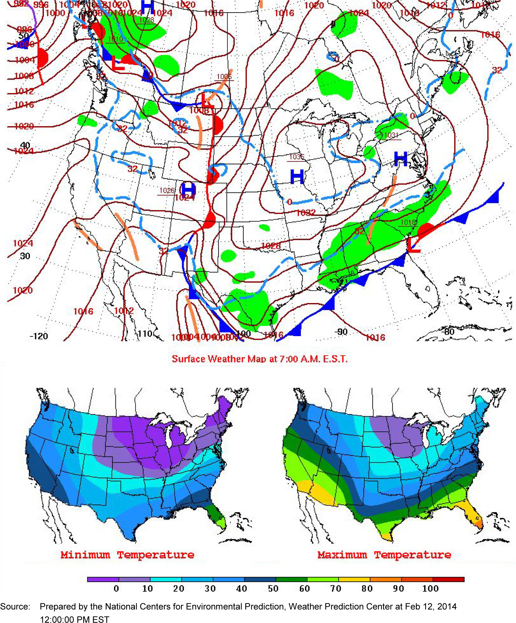
Figure 8-3 shows the surface weather map and daily minimum and maximum temperatures for February 11, 2014, the day beginning the filter pack sampling period with the highest aggregated 7-day SO2 concentrations in first quarter. The map shows a cold high pressure system over the eastern United States. Minimum temperatures below 10° Fahrenheit (F) covered a significant portion of the country. Several days during first quarter 2014 were characterized by very cold air extending from the Great Plains to the eastern seaboard.
Deer Creek, OH (DCP114)
Figure 8-3 Surface Weather Map and Daily Minimum and Maximum Temperature (°F) Maps for February 11, 2014
 Download Figure
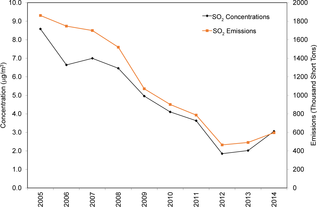
Figure 8-4 shows the trends in composite mean first quarter SO2 concentrations and emissions over the 10-year period 2005 through 2014. The increase in the SO2 concentrations for first quarter 2014 with respect to 2012 and 2013 concentrations is evident. The two time series suggest a corresponding relationship between emissions and concentrations.
Figure 8-4 Trend in Composite First Quarter Mean SO2 Concentrations and SO2 Emissions
 Download Figure
Even though quarterly mean SO42- concentrations measured in first quarter 2014 in the eastern United States were about the same as first quarter and fourth quarter 2013 levels (Amec Foster Wheeler, 2014a), the SO42- concentrations measured during the fourth week of the quarter were unusually low. Typically, SO42- collected on the CASTNET Teflon filter is higher than the fraction of SO2 collected on the nylon filter. However, during the fourth week of first quarter 2014, 21 sites sampled lower SO42- concentrations than the fraction of SO2 measured using the nylon filter. These unusual measurements do occur, though rarely, during extreme cold.
Figure 8-5 shows ratios of CASTNET 2014 week 4 SO42- concentrations to 2014 first quarter mean concentrations and ratios of historical (2005–2013) week 4 mean SO42- concentrations to historical (2005–2013) first quarter mean concentrations. Analysis of first quarter 2014 data shows that 15 sites measured ratios less than 0.5 while the historical data show that week 4 concentrations were typically closer to the quarterly mean values. The extremely cold weather affected formation of particulate SO42- concentrations negatively because oxidation of SO2 to SO42- is decreased with lower temperatures, lower O3 concentrations, and reduced photochemical reactions. In other words, the cold dry air and lower O3 levels during the week of the vortex had a significant negative effect on the formation of SO42- particles.
Figure 8-5 Ratios of 2014 Week 4 SO42- Concentrations to First Quarter 2014 Mean SO42- Concentrations and Historical (2005–2013) Week 4 Mean SO42- Concentrations to First Quarter Historical (2005–2013) Mean SO42- Concentrations
Download Figure
Chapter 9: Atmospheric Nitrogen Deposition
CASTNET was designed to provide estimates of the dry deposition of sulfur and nitrogen pollutants across the United States. To assess the status of dry and total deposition of nitrogen for 2014, CASTNET used the NADP Total Deposition Hybrid Method (TDEP) to estimate dry deposition. TDEP combines measured pollutant concentrations with output from the Community Multiscale Air Quality modeling system. TDEP used precipitation chemistry measurements at NADP/NTN sites and precipitation amounts from the Parameter-elevation Regressions on Independent Slopes Model to estimate wet deposition. Total deposition was calculated as the sum of estimated dry and wet deposition. See Chapter 10, “Atmospheric Sulfur Deposition,” for additional information on TDEP estimates of dry and wet deposition.
Gaseous and particulate nitrogen pollutants are deposited to the environment through dry and wet atmospheric processes. A principal goal of CASTNET is to estimate the rate of dry deposition from the atmosphere to sensitive ecosystems. The NADP TDEP approach (EPA, 2015b; Schwede and Lear, 2014) combines monitoring data with output from the CMAQ modeling system (Byun and Schere, 2006) to estimate dry deposition. Air quality measurements are obtained from CASTNET, AMoN, and the Southeastern Aerosol Research and Characterization (SEARCH) Network. The TDEP method gives priority to measurement data from air quality monitoring sites when available and to CMAQ output in areas where monitoring data are not available. In addition, CMAQ provides modeled data for species that are not routinely measured. The TDEP method and its recent updates are discussed on the TDEP website. See also the NADP Fact Sheet, “Hybrid Approach to Mapping Total Deposition.”
TDEP estimates wet deposition using PRISM to develop a continuous grid of precipitation data. PRISM uses terrain elevation, slope, and aspect and climatic measurements to estimate precipitation on a 4-kilometer resolution grid. Pollutant concentrations in precipitation, which were estimated for the PRISM grid, were provided by NADP/NTN. The concentration and precipitation grids were merged in order to estimate pollutant wet deposition rates. Wet deposition rates for CASTNET sites were estimated from the four nearest grid cell values. Estimates of dry and wet deposition were added to obtain estimates of total deposition, which are presented on the maps in this chapter as kilograms per hectare per year (kg ha -1 yr -1).
Nitrogen Deposition
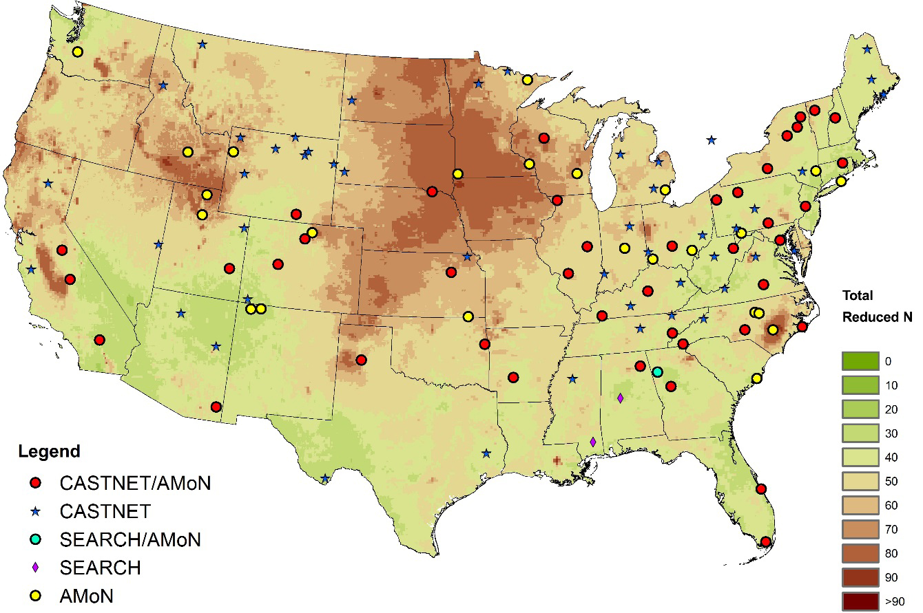
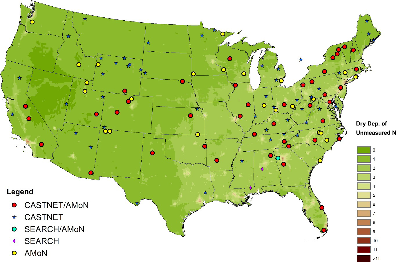
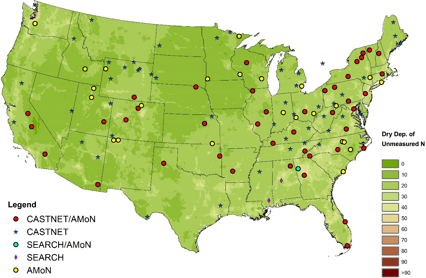
Figure 9-1 illustrates TDEP estimates of dry fluxes of nitrogen (as N) for 2014. The magnitude of the deposition fluxes is illustrated by the shading in the figure legend. A map of deposition of total N for 2014 is given in Figure 9-2. The percentage of deposition of total N due to deposition of dry N is shown in Figure 9-3. A TDEP map of reduced N species for 2014 is given in Figure 9-4. Figure 9-5 gives the percentage of reduced N species from dry deposition. Deposition of N species that are not routinely measured but are estimated by TDEP are shown in Figure 9-6. The percentage of total deposition of N that is not measured directly but is calculated by TDEP is shown in Figure 9-7.
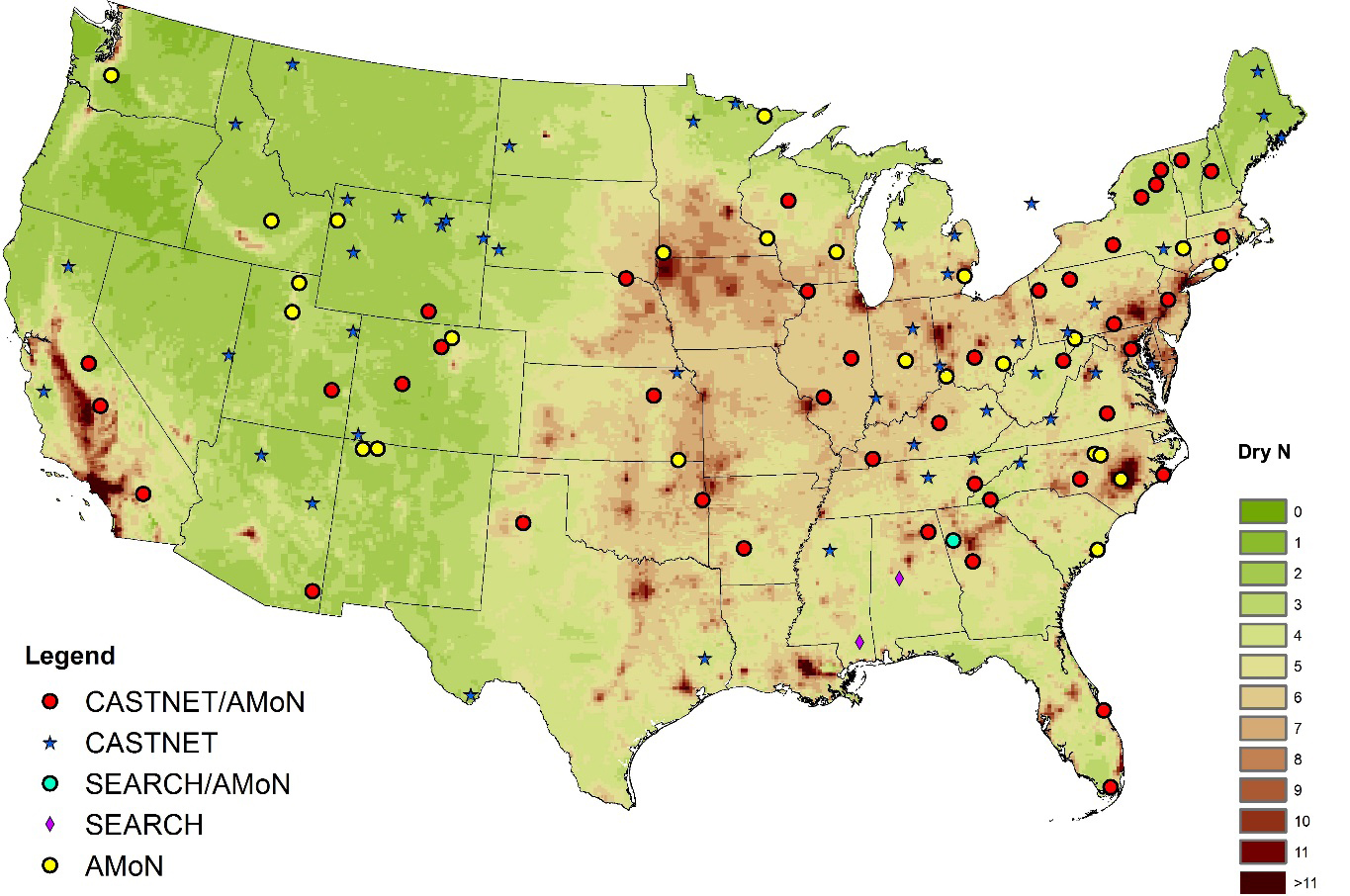
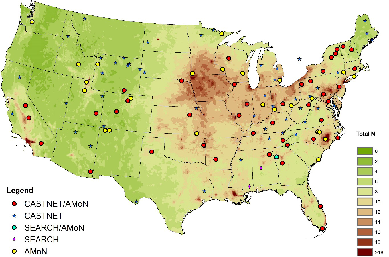
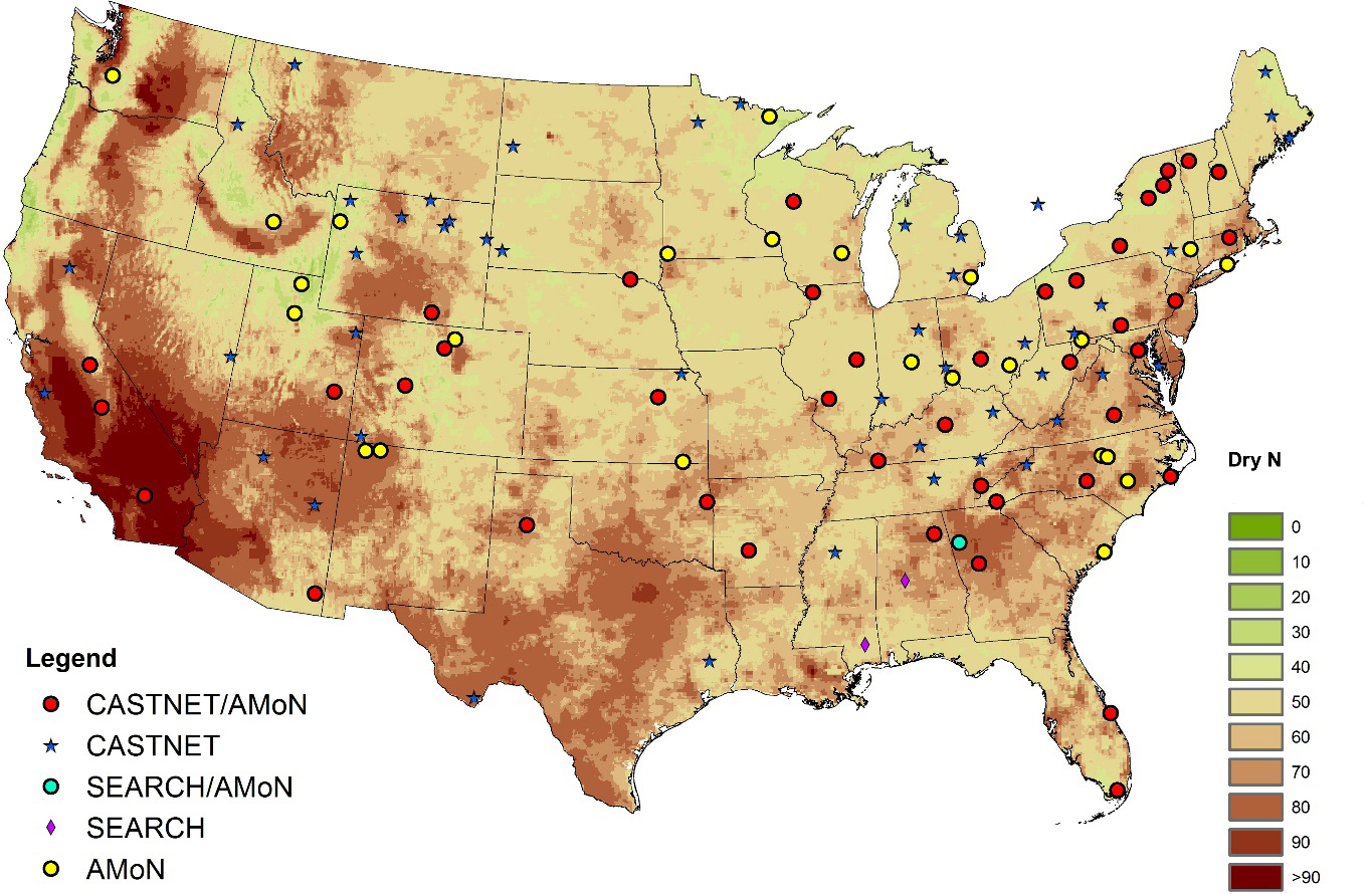

Figure 9-5 TDEP Percent of Total Deposition of Reduced N Species from Dry Deposition for 2014
 Download Figure
Figure 9-6 TDEP Deposition of N Species (kg ha -1 yr -1) not Routinely Measured for 2014
 Download Figure
Chapter 10: Atmospheric Sulfur Deposition
CASTNET was designed to provide estimates of the dry deposition of sulfur and nitrogen pollutants across the United States. CASTNET used the NADP TDEP to assess the status of dry and wet deposition of sulfur for 2014. Total deposition was calculated as the sum of estimated dry and wet deposition. See Chapter 9, “Atmospheric Nitrogen Deposition,” for additional information on TDEP estimates of dry and wet deposition.
Gaseous and particulate sulfur pollutants are deposited to the environment through dry and wet atmospheric processes. A principal goal of CASTNET is to estimate the rate of dry deposition flux from the atmosphere to sensitive ecosystems. The NADP TDEP approach (EPA, 2015b; Schwede and Lear, 2014) was used to estimate dry and wet deposition of sulfur. Estimates of dry and wet deposition were summed to obtain estimates of total deposition rates of sulfur pollutants across the United States.
Sulfur Deposition
Figure 10-1 shows a map of TDEP-modeled estimates of dry sulfur (as S) fluxes for 2014. The magnitude of the deposition fluxes is illustrated by the shading in the figure legend. A map of estimates of total deposition of S is provided in Figure 10-2. The percentage of total deposition of S due to dry deposition is shown in Figure 10-3.
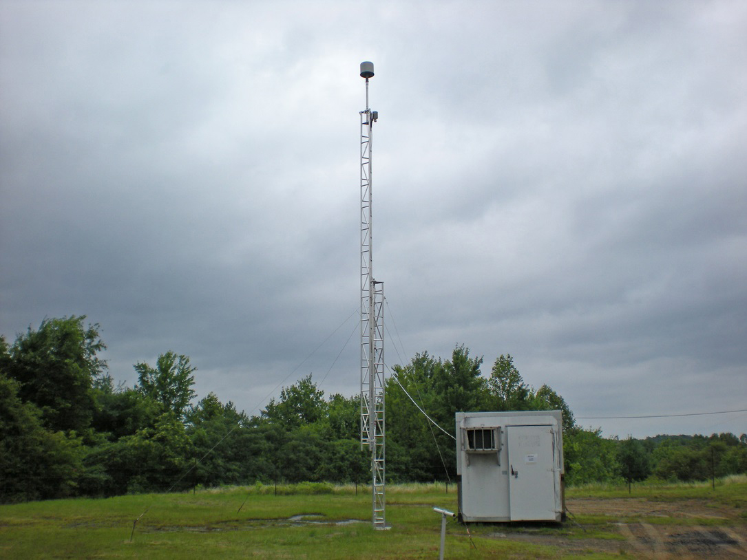
Crockett, KY (CKT136)
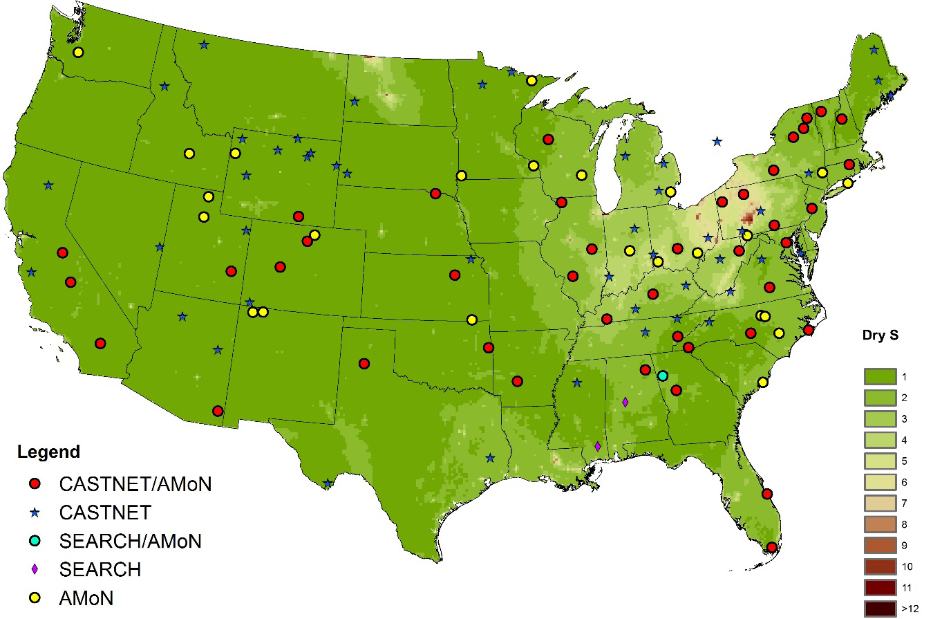
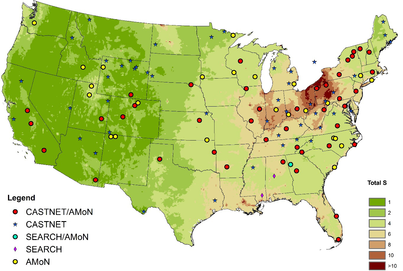
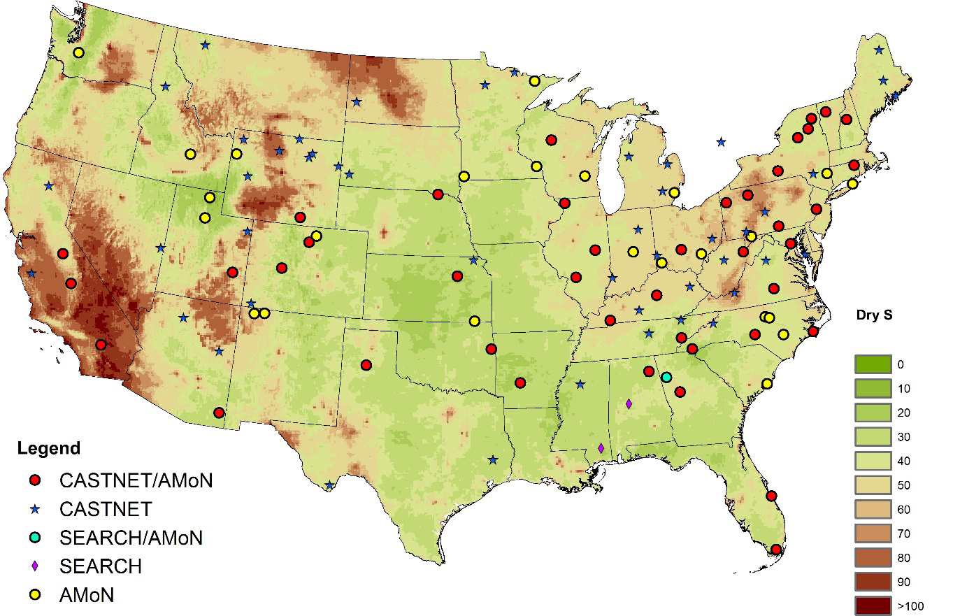
Chapter 11: Trends in Atmospheric Deposition
NADP’s TDEP was used to assess the status of dry and total deposition for 2014. TDEP was used to simulate deposition of both nitrogen and sulfur for 2014 (Chapters 9 and 10) and to estimate trends for the period 2000 through 2014. For comparison, trends in deposition were also estimated using the Multi-Layer Model (MLM)/Bowker/PRISM approach that has been used in recent CASTNET annual reports (see https://www.epa.gov/castnet). The two approaches were also compared by calculating and plotting estimates of 3-year mean dry and total deposition of nitrogen and sulfur and their annual percent changes from 2000–2002, the first 3-year period of the trends assessment, through 2012–2014. The 3-year mean TDEP estimates of total deposition of nitrogen aggregated over the eastern reference sites declined by 30 percent over the period from 2000–2002 to 2012–2014. Three-year mean total deposition of nitrogen estimated for the 16 western reference sites declined by 15 percent. Estimates of total deposition of sulfur declined 69 percent for the eastern reference sites and by 24 percent at the western reference sites. In 2014, sulfur and nitrogen total deposition estimates were at or near historic lows.
Tables 11-1 and 11-2 summarize dry and total deposition estimates and 15-year percent changes based on the TDEP and MLM box plots, which are shown in Figures 11-1 through 11-8. TDEP dry and total deposition estimates of N for CASTNET eastern reference sites were higher than the corresponding MLM estimates. This is expected because the TDEP/CMAQ modeling systems include additional N inputs not used in the MLM estimates. For example, TDEP 3-year mean estimates of total deposition of N for CASTNET eastern reference sites for 2000–2002 and 2012–2014 were 13.0 and 9.1 kg ha -1 yr -1, respectively, while MLM 3-year average estimates of total N deposition for the same periods were 7.2 and 5.3 kg ha -1 yr -1, respectively. However, the TDEP deposition estimates of dry and total S were also higher than eastern MLM results. TDEP 3-year mean estimates of total deposition of S for 2000–2002 and 2012–2014 were 15.5 and 4.8 kg ha -1 yr -1, respectively, while MLM 3-year mean deposition estimates of total S for the same periods were 9.3 and 3.8 kg ha -1 yr -1, respectively. The higher TDEP S fluxes are unexpected but perhaps are due to the difference in calculation of higher aerodynamic resistance in CMAQ versus MLM. The TDEP method and its recent updates are discussed by Schwede and Lear (2014) and on the TDEP website. See also the NADP Fact Sheet, “Hybrid Approach to Mapping Total Deposition,” (NADP/Total Deposition Science Committee, 2015). The MLM/Bowker/PRISM estimates are described by Bowker et al. (2011) and are summarized in the CASTNET 2013 Annual Report (Amec Foster Wheeler, 2015a).
Table 11-3 presents the ratios of TDEP to MLM dry and total deposition estimates for CASTNET eastern and western reference sites for the 2000–2002 and 2012–2014 periods. The table shows TDEP deposition rates were much higher than deposition rates estimated by the MLM, despite the similarity in the patterns of the 3-year mean percent changes over the period 2000 through 2014. In 2012–2014, TDEP estimates of total deposition of N at eastern sites were 1.7 times higher than eastern MLM results, and estimates of total deposition of S were about 1.3 times higher than MLM results. The TDEP/CMAQ modeling systems include emissions and concentrations that are not included in the MLM system. For example, TDEP includes NH3 emissions and measurements and trace nitrogen species that are not routinely measured. The MLM simulations were based on CASTNET air quality measurements.
Table 11-1 Summary of TDEP Trends in Deposition of Nitrogen and Sulfur
| Dry Dep of Nitrogen
(kg ha -1 yr -1) |
Total Dep of Nitrogen
(kg ha -1 yr -1) |
Percent of Total from N Dry Dep | Dry Dep of Sulfur (kg ha -1 yr -1) | Total Dep of Sulfur (kg ha -1 yr -1) | Percent of Total from S Dry Dep | |
|---|---|---|---|---|---|---|
| TDEP Eastern Sites | ||||||
| 2000–2002 | 7.9 | 13.0 | 60% | 9.8 | 15.5 | 57% |
| 2012–2014 | 4.9 | 9.1 | 53% | 2.0 | 4.8 | 39% |
| Percent Change | -39% | -30% | -79% | -69% | ||
| TDEP Western Sites | ||||||
| 2000–2002 | 3.2 | 4.6 | 67 | 0.7 | 1.4 | 50% |
| 2012–2014 | 2.3 | 3.9 | 60 | 0.5 | 1.1 | 46% |
| Percent Change | -26% | -15% | -34% | -24% | ||
Table 11-2 Summary of MLM Trends in Deposition of Nitrogen and Sulfur
| Dry Dep of Nitrogen
(kg ha -1 yr -1) |
Total Dep of Nitrogen
(kg ha -1 yr -1) |
Percent of Total from N Dry Dep | Dry Dep of Sulfur (kg ha -1 yr -1) | Total Dep of Sulfur (kg ha -1 yr -1) | Percent of Total from S Dry Dep | |
|---|---|---|---|---|---|---|
| MLM Eastern Sites | ||||||
| 2000–2002 | 2.1 | 7.2 | 29% | 3.5 | 9.3 | 35% |
| 2012–2014 | 1.0 | 5.3 | 19% | 1.0 | 3.8 | 25% |
| Percent Change | -53% | -27% | -71% | -59% | ||
| MLM Western Sites | ||||||
| 2000–2002 | 0.9 | 2.3 | 39% | 0.3 | 0.9 | 28% |
| 2012–2014 | 0.6 | 2.1 | 28% | 0.2 | 0.8 | 25% |
| Percent Change | -33% | -8% | -27% | -18% | ||
Table 11-3 Ratio of TDEP to MLM Deposition Estimates of Nitrogen and Sulfur
| Dry Dep of Nitrogen | Total Dep of Nitrogen | Dry Dep of Sulfur | Total Dep of Sulfur | |
|---|---|---|---|---|
| TDEP/MLM Eastern Sites | ||||
| 2000–2002 | 3.8 | 1.8 | 2.8 | 1.7 |
| 2012–2014 | 4.9 | 1.7 | 2.0 | 1.3 |
| TDEP/MLM Western Sites | ||||
| 2000–2002 | 3.5 | 2.0 | 2.8 | 1.5 |
| 2012–2014 | 3.9 | 1.8 | 2.5 | 1.4 |
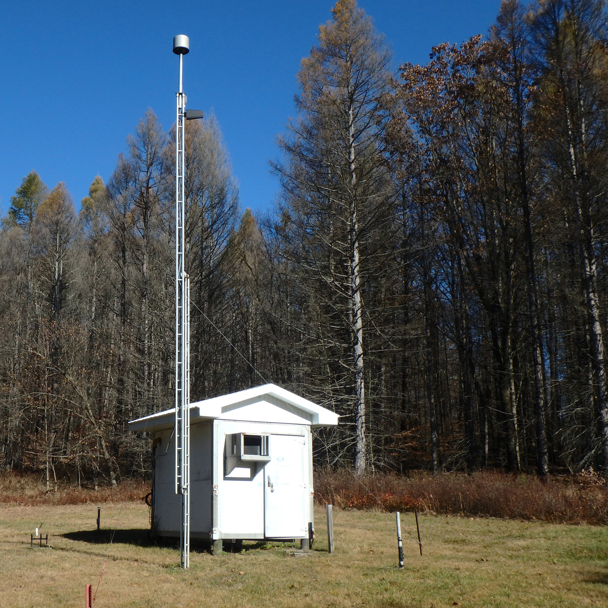
Laurel Hill State Park, PA (LRL117)
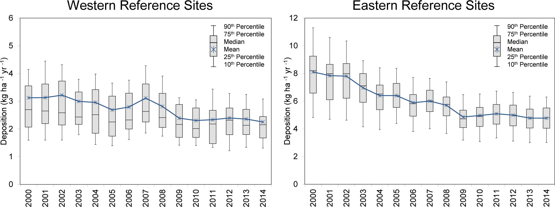
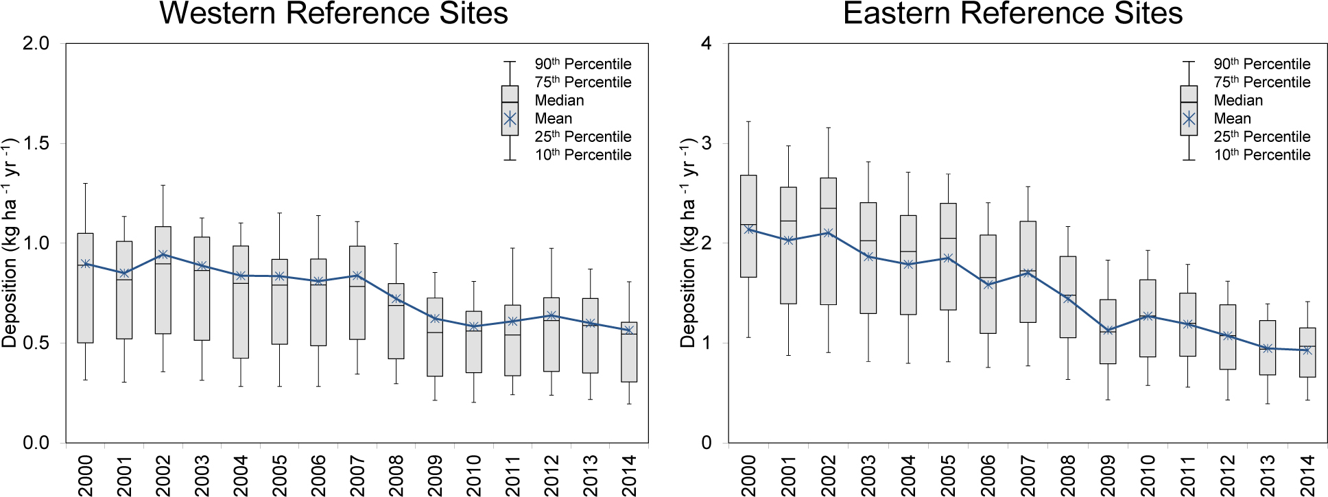
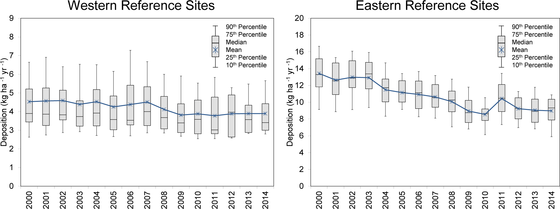
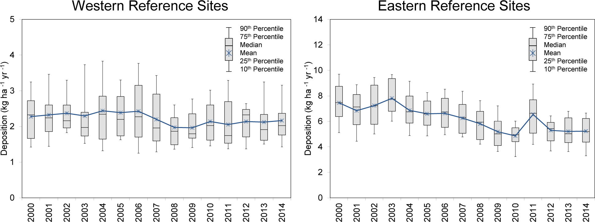
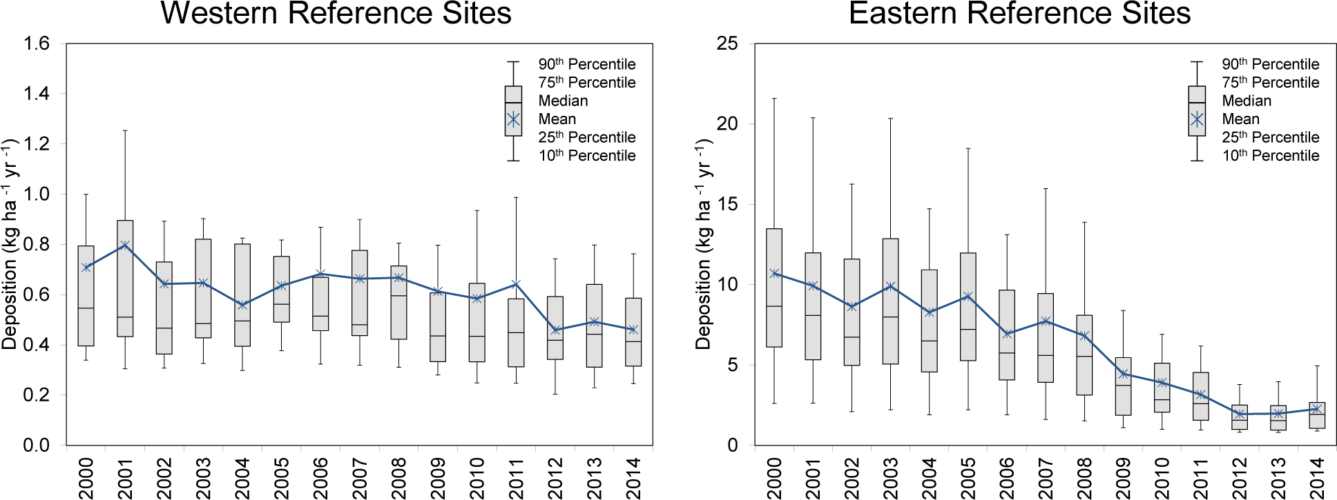
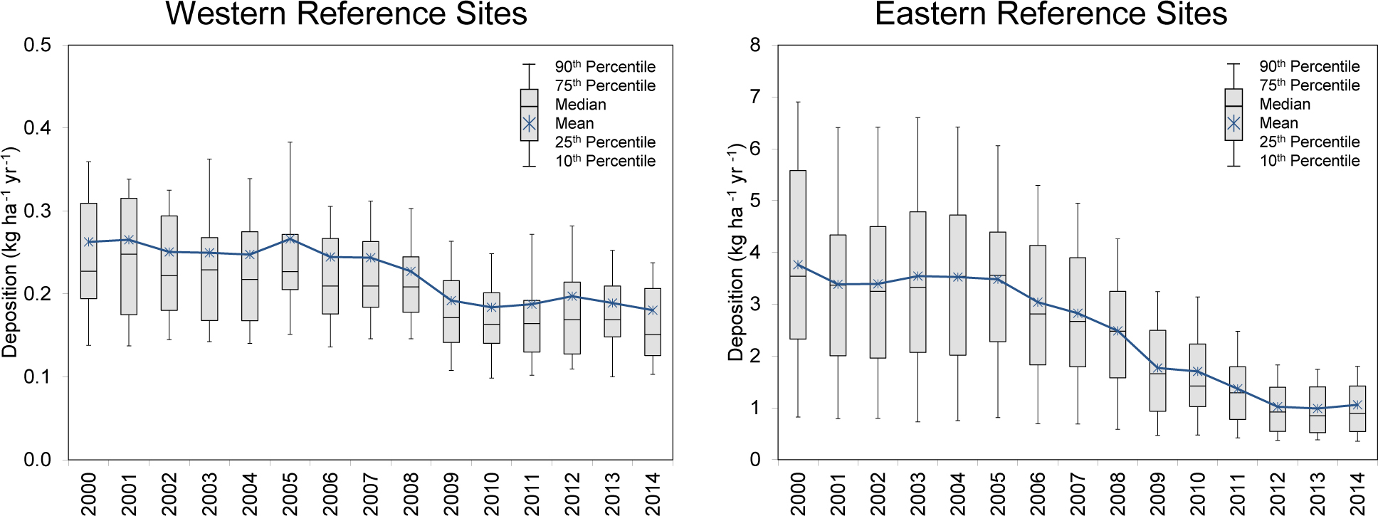
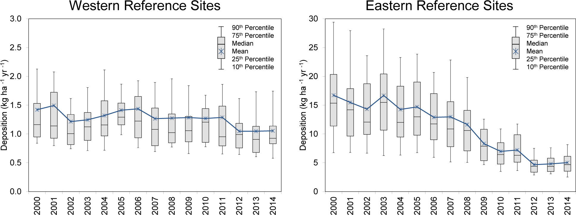
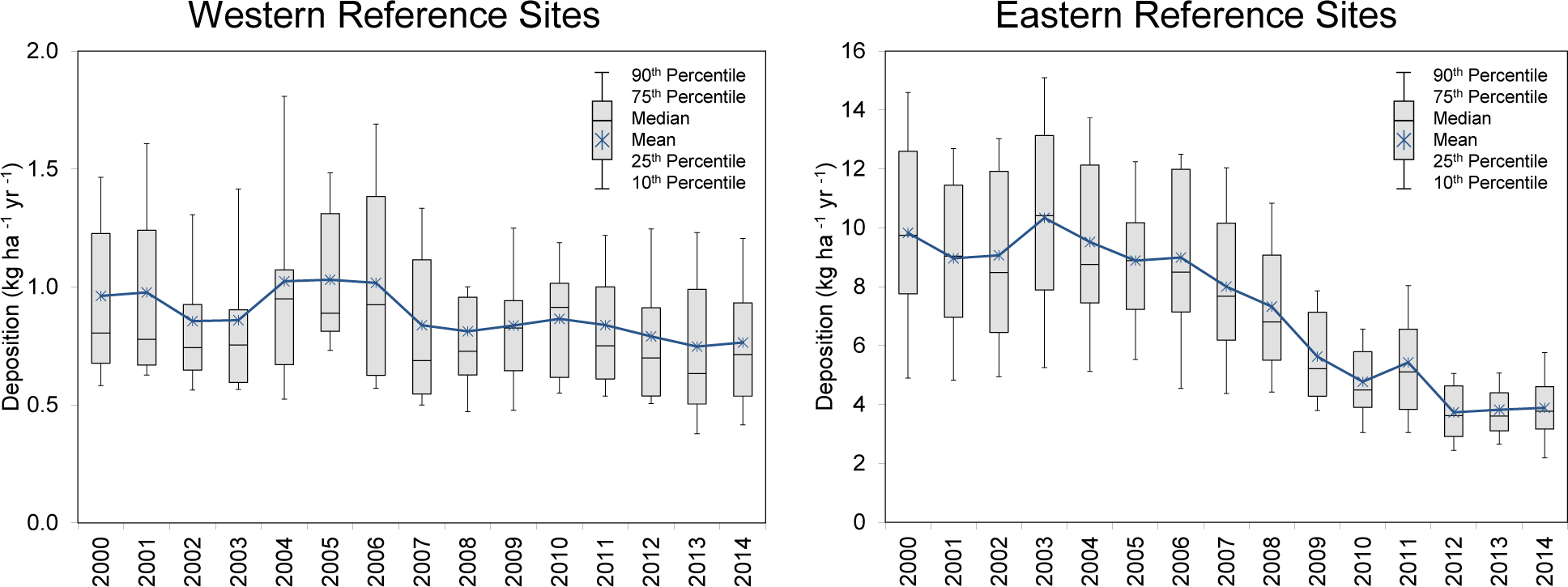
Figures 11-9 through 11-12 show year-by-year percent changes in TDEP and MLM 3-year mean dry and total deposition estimates of N and S. Estimates of total deposition of S have been reduced more quickly and effectively at the eastern reference sites than the western sites, although reductions in deposition of both N and S have been realized at the western reference sites as well.
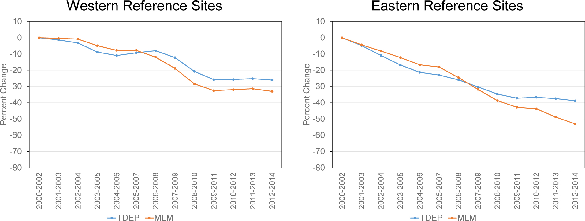
Figure 11-10 Percent Change in 3-year Mean TDEP and MLM Total Deposition of Nitrogen
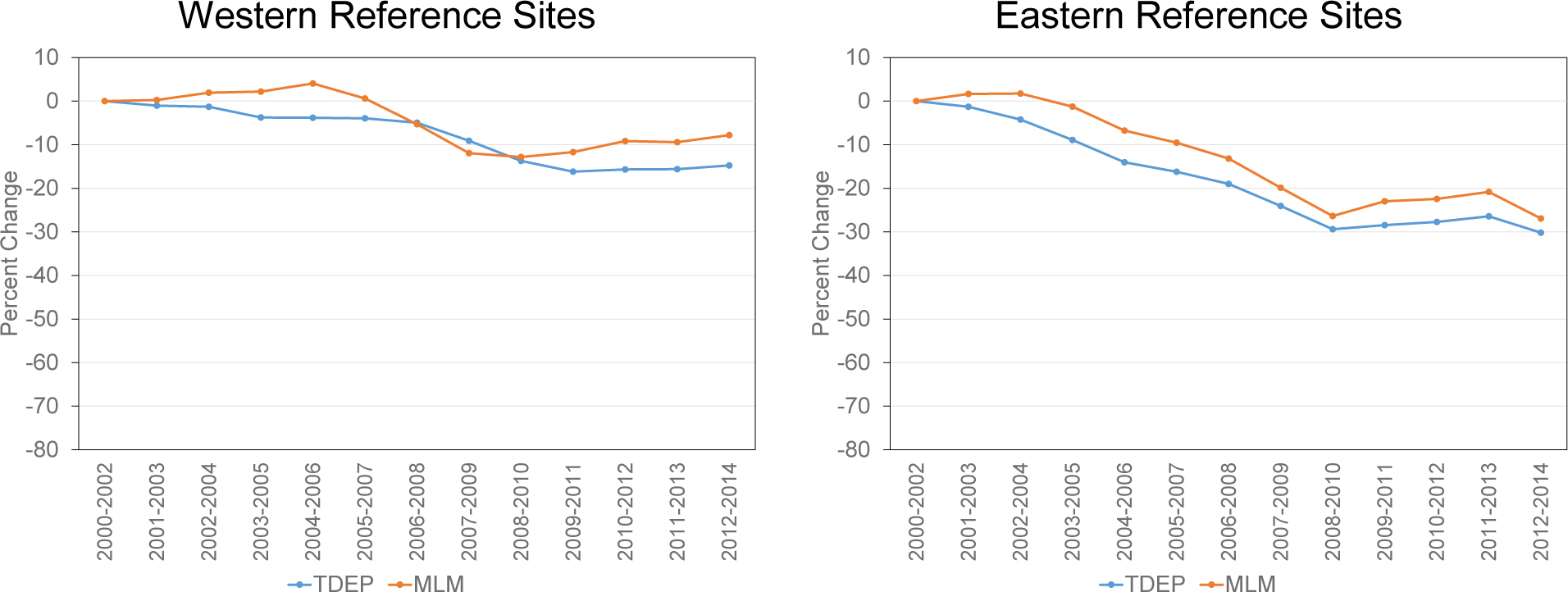 Download Figure
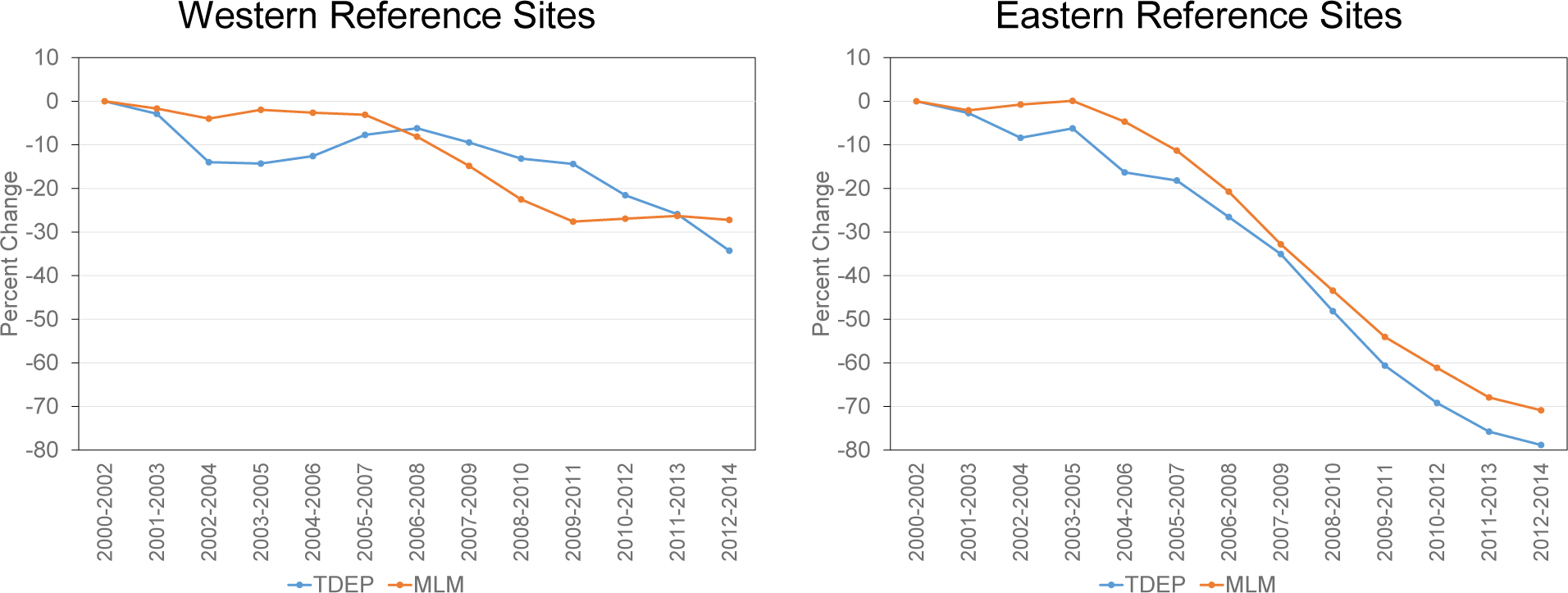
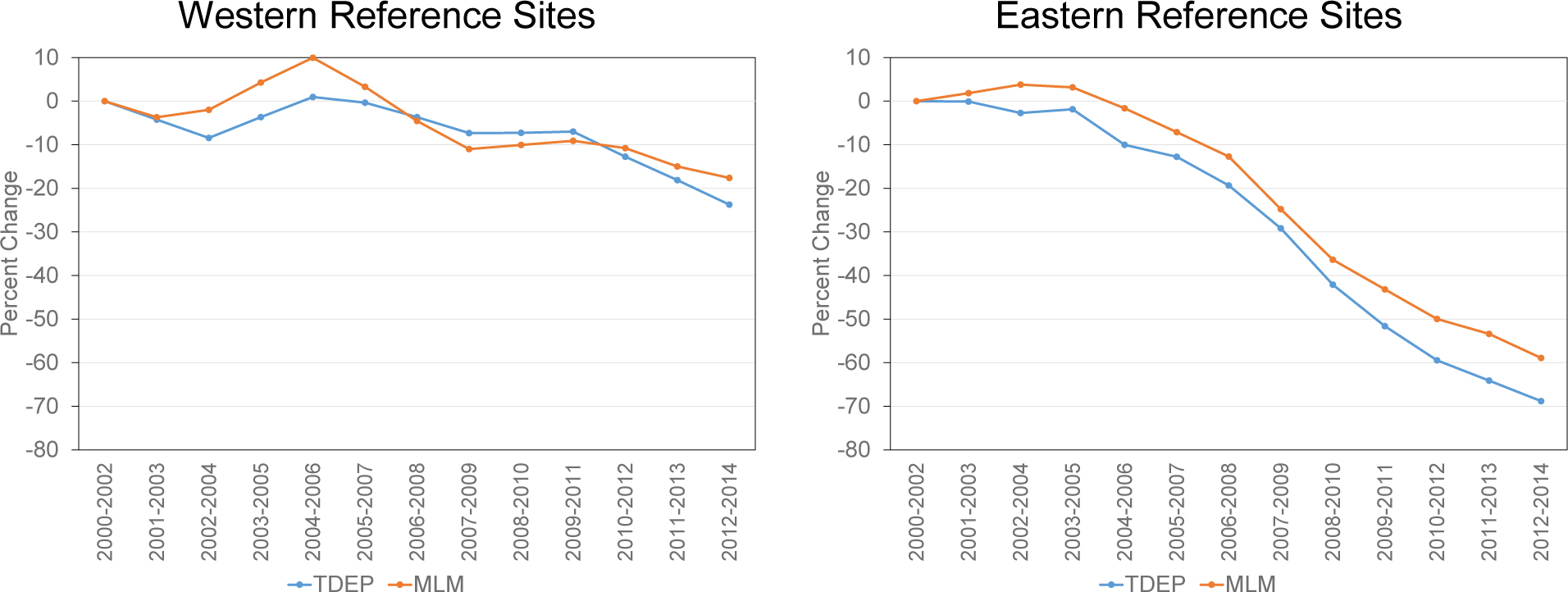
Chapter 12: Development of Maps of Critical Loads for the United States
Information on critical loads is an important tool for assessing the risk to ecosystems due to acidic deposition. The primary forum for critical loads research and development coordination in the United States has been NADP’s Critical Loads of Atmospheric Deposition Science Committee (CLAD). Commencing in 2010, the CLAD Focal Center Utility Study, i.e., “FOCUS Pilot Study,” assembled and synthesized empirical and calculated critical loads data and information from regional and national-scale projects. The first round of critical load data synthesis was used for an unofficial submission to the United Nations Economic Commission for Europe Coordinating Center on Effects. This information delivery represented the interests of a growing critical loads science community in the United States. CLAD members and others submitted data to this cooperative effort to share information to improve methods for estimating, calculating, mapping, interpreting, and refining critical loads. Since then, the CLAD critical load database has been improved and additional values have been added.
Air pollution emitted from a variety of sources eventually deposits out of the air through precipitation or dry deposition into natural environments. Air pollutants cause negative effects, such as acidification, soil nutrient imbalances, and loss of biodiversity. Certain ecosystems in national parks are particularly vulnerable to pollutant deposition, including high elevation lakes and streams, alpine meadows, sugar maple forests, and desert shrublands. The information on critical loads has provided a valuable tool for assessing ecosystem health and guiding resource management decisions.
“Critical load” is a term used to describe the amount of pollution initiating harmful changes in sensitive ecosystems. A critical load is defined as “the quantitative estimate of an exposure to one or more pollutants below which significant harmful effects on specified sensitive elements of the environment do not occur according to present knowledge” (Nilsson and Grennfelt, 1988).
Critical load data can be used to assess a variety of ecosystem responses to air pollution deposition including changes in aquatic and terrestrial plant diversity, soil nutrient levels, and fish health. Some parts of an ecosystem are more sensitive than others; therefore, the effects of pollutant loading will differ within ecosystems. For example, critical loads to maintain healthy fish in lakes and streams are different than those for soil conditions needed to sustain healthy forests. When critical loads are exceeded, i.e., when deposition is greater than the critical load, the environmental effects can cascade. For instance, excess nitrogen can act as a fertilizer, encouraging exotic grass species to establish in desert ecosystems in sufficient densities to fuel wildfires in areas not adapted to fire.
This chapter presents brief synopses of the CLAD estimates of critical loads of sulfur and nitrogen across the United States and includes information from the CLAD FOCUS Pilot Study (Blett et al., 2014) and example maps (Lynch et al., 2015).
The CLAD FOCUS project was instituted to develop and implement a process for calculating and mapping critical loads within the United States. The FOCUS Pilot Study assembled and synthesized calculated and empirical critical loads information and data from several regional and national-scale projects in order to prepare national maps of critical loads. The CLAD critical loads database includes:
- Surface water/aquatic critical loads of acidity: Mass balance steady-state surface water models, e.g., Steady-State Water Chemistry model, were used to calculate critical loads for locations with available water chemistry measurements.
- Forest ecosystem/terrestrial critical loads of acidity: Simple mass balance equations were used to calculate critical loads based on a 1 square kilometer (km 2 ) grid across forested lands in the lower 48 states (McNulty et al., 2007; Duarte et al., 2013).
- Empirical critical loads for nitrogen: The methods and results of Pardo et al. (2011b) were used to estimate critical loads for fungi, herbaceous vegetation, forests, and nitrate leaching. Critical loads estimated by Geiser et al. (2010) were used to characterize lichen. These critical loads were mapped on a 4 km 2 grid.
Steady-state critical loads for acidity of surface waters for approximately 12,500 streams and lakes are included in the CLAD database. The critical loads data were obtained from agencies such as the USGS, U.S. Forest Service (USFS) Air Program, and EPA (see Table 2 in Blett et al., 2014). Other sources include regional lake and national stream surveys. The threshold used for all aquatic critical loads estimates was an acid neutralizing capacity (ANC) of 50 microequivalents per liter (μeq/L) with the exception of the average critical loads for sulfur and nitrogen shown in Figure 12-1, which used an ANC threshold of 50 μeq/L for eastern locations and an ANC threshold of 20 μeq/L for western locations. Figure 12-1 shows average critical loads of surface sulfur and nitrogen acidity in milliequivalents per square meter per year (meq m -2 yr -1) based on 12 kilometer (km) x 12 km grid cells. Figure 12-1 excluded values with a runoff rate greater than 0.15 millimeters per year (mm/yr). Lynch et al. (2015) also shows maps with 12 km x 12 km and 36 km x 36 km grids based on average and 10th percentile critical loads.

Terrestrial critical loads of acidity were calculated by McNulty et al. (2007) and Duarte et al. (2013) for forested lands across the continental United States. A steady-state simple mass balance model (UBA, 2004) was used for the estimates. Figure 12-2 depicts average critical loads of nitrogen acidity as kg ha -1 yr -1 for either a 1 km x 1 km or a 12 km x 12 km grid system. The base cation to aluminum ratio for forest soils was used as the critical chemical criterion. A ratio of 1.0 molar equivalents per hectare per year (eq ha -1 yr -1) was used for deciduous forests and a ratio of 10.0 eq ha -1 yr -1 for coniferous forests.
The database of empirical critical loads of nitrogen was created using information and data from Pardo et al. (2011b) and Geiser et al. (2010). The methods of Pardo et al. (2011b) were used to calculate critical loads for fungi, herbaceous vegetation, forests, and nitrate leaching. Critical loads estimated by Geiser et al. (2010) were used to characterize lichen. Table 4 given in Blett et al. (2014) summarizes the empirical critical loads for nitrogen. Figure 12-3 shows empirical critical loads of nitrogen for forest ecosystems. Figure 12-4 depicts critical loads of nitrogen for herbaceous plants and shrubs, and Figure 12-5 gives critical loads for lichen.
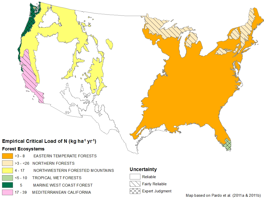
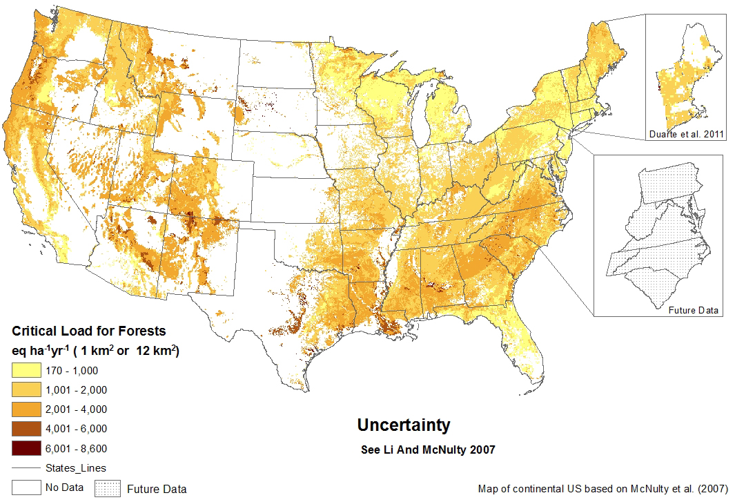
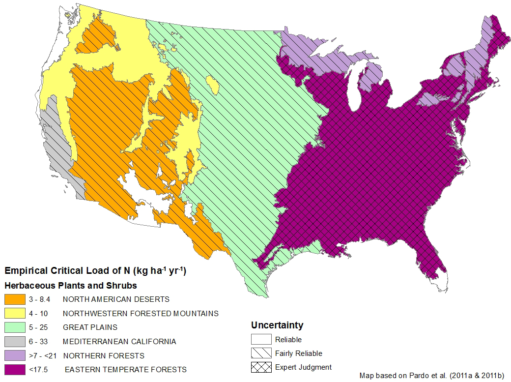
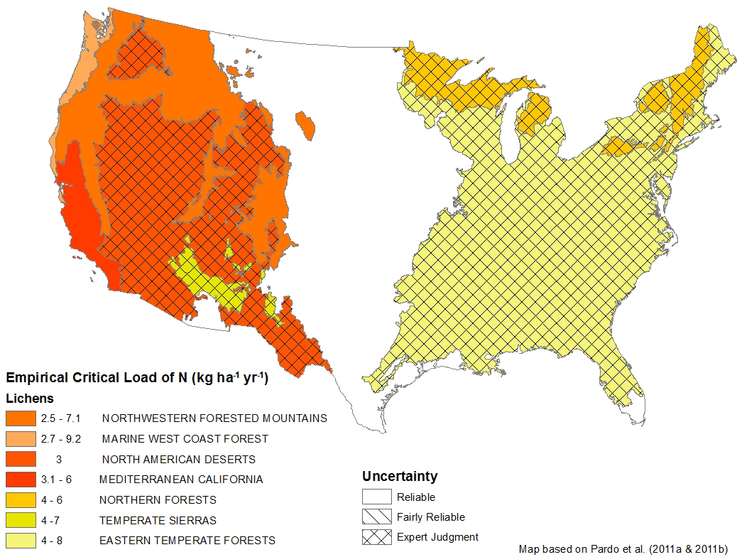
The maps in Figures 12-1 through 12-5 represent the first steps in the development of national critical loads information. However, significant uncertainties remain in these approximations, including the following:
- The surface water critical loads are considered reasonable because they are based on actual water quality measurements at over 12,000 sites, some for several years. Despite the extensive database, the critical load values are based on uncertain input data, for example, estimates of the weathering rate in a watershed.
- The forest ecosystem critical loads are approximate. These are the first estimates of forest soil critical loads nationwide. Forest ecosystem critical loads need to be updated using a new weathering rate model. Yet these are the best available estimates nationwide.
- The empirical critical loads for nitrogen-estimated uncertainties are shown on the maps as “reliable,” “fairly reliable,” or “expert judgment.” These critical loads are considered the weakest of the three databases. The most uncertain element is the mapping. A wide range of critical loads is applied to a large area without considering the area’s receptors or communities. Pardo is investigating more site-specific mapping in order to improve spatial coverage.
FOCUS Phase II is underway to improve critical load estimates. The Phase II work includes reviewing ecosystem research and monitoring, deposition monitoring and modeling, critical loads model parameterization, database infrastructure, and management and policy support (Blett et al. 2014). The end products will include updated maps of critical loads for the United States.
References
Amec Foster Wheeler Environment & Infrastructure, Inc. 2015a. Clean Air Status and Trends Network (CASTNET) 2013 Annual Report. Prepared for U.S. Environmental Protection Agency (EPA), Office of Air and Radiation, Clean Air Markets Division, Washington, DC. Contract No. EP-W-15-003. Gainesville, FL.
Amec Foster Wheeler Environment & Infrastructure, Inc. 2015b. Clean Air Status and Trends Network (CASTNET) Fourth Quarter 2014 Data Report. Prepared for U.S. Environmental Protection Agency (EPA), Office of Air and Radiation, Clean Air Markets Division, Washington, DC. Contract No. EP-W-15-003. Gainesville, FL.
Amec Foster Wheeler Environment & Infrastructure, Inc. 2015c. Clean Air Status and Trends Network (CASTNET) Third Quarter 2014 Data Report. Prepared for U.S. Environmental Protection Agency (EPA), Office of Air and Radiation, Clean Air Markets Division, Washington, DC. Contract No. EP-W-09-028. Gainesville, FL.
Amec Foster Wheeler Environment & Infrastructure, Inc. 2014a. Clean Air Status and Trends Network (CASTNET) First Quarter 2014 Data Report. Prepared for U.S. Environmental Protection Agency (EPA), Office of Air and Radiation, Clean Air Markets Division, Washington, DC. Contract No. EP-W-09-028. Gainesville, FL.
Amec Foster Wheeler Environment & Infrastructure, Inc. 2014b. Clean Air Status and Trends Network (CASTNET) Second Quarter 2014 Data Report. Prepared for U.S. Environmental Protection Agency (EPA), Office of Air and Radiation, Clean Air Markets Division, Washington, DC. Contract No. EP-W-09-028. Gainesville, FL.
Amec Foster Wheeler Environment & Infrastructure, Inc. 2013. Clean Air Status and Trends Network (CASTNET) Quality Assurance Project Plan (QAPP) Revision 8.1. Prepared for U.S. Environmental Protection Agency (EPA), Office of Air and Radiation, Clean Air Markets Division, Washington, DC. Contract No. EP-W-09-028. Gainesville, FL. https://java.epa.gov/castnet/documents.do.
Baumann, K., Williams, E. J., Olson, J. A., Harder, J. W., and Fehsenfeld F. C. 1997. Meteorological Characteristics and Spatial Extent of Upslope Events during the 1993 Tropospheric OH Photochemistry Experiment. J. Geophys. Res., 102(D5), 6199–6213, doi:10.1029/96JD03251.
Baumgardner, R.E., Rogers, C.M., Puchalski, M.R., Lavery, T.F., Mishoe, K.P., Price, G.L., and Hall, N.H. 2014. Measurements of Atmospheric NH3, NO7/NOx, and NO2 and Deposition of Total Nitrogen at the Beaufort, NC CASTNET Site (BFT142). U.S. Environmental Protection Agency Office of Research and Development, Research Triangle Park, NC 27711. EPA/600-R-14/182.
Blett, T.F., Lynch, J.A., Pardo, L.H., Huber, C., Haeuber, R., Pouyat, R. 2014. FOCUS: A Pilot Study for National-Scale Critical Loads Development in the United States. Environmental Science & Policy. 38 (2014) 225-236. February 3.
Bowker, G.E., Schwede, D.B., Lear, G.G., Warren-Hicks, W.J., and Finkelstein, P.L. 2011. Quality Assurance Decisions with Air Models: A Case Study of Imputation of Missing Input Data Using EPA’s Multi-Layer Model. Water, Air, & Soil Pollution 223:391-402. doi: 10.1007/s11270-011-0832-7.
Byun, D. and Schere, K.L. 2006. Review of the Governing Equations, Computational Algorithms, and Other Components of the Models-3 Community Multiscale Air Quality (CMAQ) Modeling System. Applied Mechanics Reviews, 59: 51-77. doi: 10.1115/1.2128636.
Duarte, N., Pardo, L.H., and Robin-Abbott, M.J. 2013. Susceptibility of Forests in the Northeastern USA to Nitrogen and Sulfur Deposition: Critical Load Exceedance and Forest Health. Water Air Soil Pollution (224). doi: 10.1007/s11270-012-1355-6.
Duarte, N., Pardo, L.H., and Robin-Abbott, M. J. 2011. Susceptibility of Forests in the Northeastern U.S. to Nitrogen and Sulfur Deposition. New England Governors/Eastern Canadian Premiers Forest mapping research project report. http://www.nrs.fs.fed.us/clean_air_water/clean_water/critical_loads/pubs/. Updated 2012: http://www.nrs.fs.fed.us/clean_air_water/clean_water/critical_loads/localresources/ docs/FHM-report2012.pdf. Accessed August 2016.
Geiser, L.H., Jovan, S.E., Glavich, D.A., Porter, M. 2010. Lichenbased Critical Loads for Atmospheric Nitrogen Deposition in Western Oregon and Washington Forests USA. Environ. Pollut. 158, 2412–2421.
Kennedy, C. 2014. Wobbly Polar Vortex Triggers Extreme Cold Air Outbreak. National Oceanic and Atmospheric Association (NOAA) Climate.gov. https://www.climate.gov/news-features/event-tracker/wobbly-polar-vortex-triggersextreme- cold-air-outbreak. Accessed August 2015.
Li, H. and McNulty, S.G. 2007. Uncertainty Analysis on Simple Mass Balance Model to Calculate Critical Loads for Soil Acidity. Environmental Pollution, Vol. 149: 315-326.
Lynch, J., Pardo L., and Huber, C. 2015. Detailed Documentation of the CLAD U.S. Critical Loads of Sulfur and Nitrogen Access Database, version 2.5. National Atmospheric Deposition Program, Illinois State Water Survey, Champaign, IL. http://nadp.sws.uiuc.edu/committees/clad/db/. Accessed August 2016.
Martin, R.S. and Baasandorj, M. 2016. A Comparison of AMoN Measurements with Localized, Arrayed Passive NH3 Samplers in Northern Utah. Presentation submitted to the National Atmospheric Deposition Program (NADP), 2016 Fall Meeting, Santa Fe, NM, Oct. 31 – Nov. 4.
McNulty, S.G., Cohen, E.C., Moore-Myers, J.A., Sullivan, T.J., and Li, H. 2007. Estimates of Critical Acid Loads and Exceedances for Forest Soils across the Conterminous United States. Environmental Pollution. 149: 281-292.
Mishoe, K.P., Rogers, C.M., Beachley, G., Puchalski, M.A., Howell, H.K., Stewart, M.O. 2015. Speciated Reactive Nitrogen Measurements using Chemiluminescence. Air & Waste Management Association (A&WMA) Extended Abstract # 386. Proceedings of the A&WMA Annual Conference & Exhibition, Raleigh, North Carolina, June 22-25.
National Atmospheric Deposition Program (NADP)/Ammonia Monitoring Network (AMoN) 2015. Ambient Ammonia Monitoring Network (AMoN) Fact Sheet. http://nadp.sws.uiuc.edu/AMoN/AMoNFactSheet.pdf. Accessed July 2015.
National Atmospheric Deposition Program (NADP)/Total Deposition Science Committee 2015. Hybrid Approach to Mapping Total Deposition. http://nadp.isws.illinois.edu/lib/brochures/tdepsheet.pdf. Accessed December 2015.
National Centers for Environmental Information, formerly known as the National Climatic Data Center. 2014. National Overview – January 2014 | State of the Climate. https://www.ncdc.noaa.gov/sotc/national/201401. Accessed August 2016.
National Centers for Environmental Information, formerly known as the National Climatic Data Center. 2013. U.S. Daily Snowfall Records set on December 6, 2013. https://www.ncdc.noaa.gov/sotc/national/201312. Accessed July 2015.
Nilsson, J., and Grennfelt, P. (Eds). 1988. Critical Loads for Sulphur and Nitrogen. UNECE/Nordic Council workshop report, Skokloster, Sweden. March 1988. Nordic Council of Ministers: Copenhagen.
North American Electric Reliability Corporation. 2014. Polar Vortex Review. September 2014. http://www.nerc.com/pa/rrm/January%202014%20Polar%20Vortex%20Review/Polar_Vo rtex_Review_29_Sept_2014_Final.pdf. Accessed October 2016.
Pardo, L.H., Fenn, M.E., Goodale, C.L., Geiser, L.H., Driscoll, C.T., Allen, E.B., Baron, J.S., et al. 2011a. Effects of Nitrogen Deposition and Empirical Nitrogen Critical Loads for Ecoregions of the United States. Ecological Applications. 21(8): 3049–3082.
Pardo, L.H., Robin-Abbott, M.J., and Driscoll, C.T. eds. 2011b. Assessment of Nitrogen Deposition Effects and Empirical Critical Loads of Nitrogen for Ecoregions of the United States. General Technical Report NRS-80. U.S. Department of Agriculture, Forest Service, Northern Research Station, Newtown Square, PA.
Puchalski, M.A, Sather, M.E., Walker, J.T., Lehmann, C.M.B., Gay, D.A., Mathew, J., and Robarge, W.P. 2011. Passive Ammonia Monitoring in the United States: Comparing Three Different Sampling Devices. J. Environ. Monit., 13:3156-67. doi: 10.1039/c1em10553a
Rice, D. 2014. A List of Record Low Temperatures Set Tuesday: Coldest Air in Decades. USA Today. http://www.usatoday.com/story/weather/2014/01/07/weather-polar-vortexcold/ 4354945/. Accessed July 2015.
Schwede, D.B. and Lear, G.G. 2014. A Novel Hybrid Approach for Estimating Total Deposition in the United States. Atmos. Environ., 92:207-220. doi: 10.1016/j.atmosenv.2014.04.008.
Sosnowski, A. 2014. Rough Winter to Lag into March for Midwest and East. http://www.accuweather.com/en/weather-news/rough-winter-to-lag-intomarch/ 23744744. Accessed March 2015.
Talbot, R., Mao, H., and Sive, B. 2005. Diurnal Characteristics of Surface Level O3 and other Important Trace Gases in New England, J. Geophys. Res., 110, D09307, doi:10.1029/2004JD005449.
UBA. 2004. Manual on Methodologies and Criteria for Modeling and Mapping Critical Loads and Levels and Air Pollution Effects, Risks and Trends. Federal Environmental Agency (Umweltbundesamt), Berlin, Germany, Online: icpmapping.org. Accessed July 2015.
U.S. Environmental Protection Agency (EPA). 2016. Final Cross-State Air Pollution Rule Update. Clean Air Markets Division. https://www.epa.gov/airmarkets/final-cross-state-air-pollutionrule- update. Accessed October 2016.
U.S. Environmental Protection Agency (EPA). 2015a. Overview of EPA’s Updates to the Air Quality Standards for Ground-level Ozone. https://www.epa.gov/sites/production/files/2015- 10/documents/overview_of_2015_rule.pdf. Accessed December 2015.
U.S. Environmental Protection Agency (EPA). 2015b. Total Deposition Estimates Using a Hybrid Approach. ftp://ftp.epa.gov/castnet/tdep/Total_Deposition_Documentation_current.pdf. Accessed June 2015.
U.S. Environmental Protection Agency (EPA). 2013a. Quality Assurance Handbook for Air Pollution Measurement Systems, Volume II, Ambient Air Quality Monitoring Program. EPA-454/B-13-003, May. http://www.epa.gov/ttnamti1/files/ambient/pm25/qa/QA-Handbook-Vol-II.pdf
U.S. Environmental Protection Agency (EPA). 2013b. Treatment of Data Influenced by Exceptional Events. https://www.epa.gov/air-quality-analysis. Accessed December 2014.
U.S. Environmental Protection Agency (EPA). 2008. National Ambient Air Quality Standards for Ozone; Final Rule. Federal Register 73, No. 60 (March). EPA-HQ-OAR-2005-0172.
U.S. Environmental Protection Agency (EPA). 1998. Guideline on Data Handling Conventions for the 8-Hour Ozone NAAQS. EPA-454/R-98-017. OAQPS, Research Triangle Park, NC 27711.
Appendix A: Locational and Operational Characteristics of CASTNET Sites
| Site ID | Site Name | Start Date | Latitude | Longitude | Elevation | Nearby NADP | Land Use | Terrain | Agency | Reference |
|---|---|---|---|---|---|---|---|---|---|---|
| ABT147, CT | Abington | 12/28/93 | 41.8405 | -72.0104 | 202 | CT15 | Urban/Agric | Rolling | EPA | |
| ACA416, ME | Acadia NP | 12/1/98 | 44.3771 | -68.2608 | 158 | ME98 | Forest | Rolling | NPS | |
| ALC188, TX | Alabama-Coushatta | 4/6/04 | 30.7016 | -94.674 | 105 | TX10 | Prairie | Rolling | EPA | |
| ALH157, IL | Alhambra | 6/28/88 | 38.869 | -89.6228 | 164 | IL46 | Agric | Flat | EPA | E |
| ANA115, MI | Ann Arbor | 6/28/88 | 42.4166 | -83.9022 | 266 | MI52 | Forest | Flat | EPA | E |
| ARE128, PA | Arendtsville | 6/28/88 | 39.9232 | -77.3079 | 266 | PA00 | Agric | Rolling | EPA | E |
| ASH135, ME | Ashland | 12/20/88 | 46.6038 | -68.4132 | 231 | ME00 | Agric | Flat | EPA | E |
| BAS601, WY | Basin | 11/6/12 | 44.28 | 108.0411 | 1242 | MT00 | Prairie | Rolling | BLM | |
| BBE401, TX | Big Bend NP | 7/18/95 | 29.3027 | 103.1778 | 1052 | TX04 | Forest | Complex | NPS | W |
| BEL116, MD | Beltsville | 11/1/88 | 39.0282 | -76.8171 | 47 | MD99 | Range | Flat | EPA | E |
| BFT142, NC | Beaufort | 12/28/93 | 34.8847 | -76.6207 | 5 | NC06 | Agric | Flat | EPA | |
| BUF603, WY | Buffalo | 11/6/12 | 44.1442 | 106.1089 | 1324 | WY99 | Prairie | Rolling | BLM | |
| BVL130, IL | Bondville | 2/9/88 | 40.052 | -88.3725 | 213 | IL11 | Agric | Flat | EPA | E |
| BWR139, MD | Blackwater NWR | 7/4/95 | 38.445 | -76.1113 | 1 | MD15 | Forest/Marsh | Coastal | EPA | |
| CAD150, AR | Caddo Valley | 10/4/88 | 34.1793 | -93.0988 | 78 | AR03 | Forest | Complex | EPA | E |
| CAN407, UT | Canyonlands NP | 1/24/95 | 38.4583 | 109.8213 | 1809 | UT09 | Desert | Complex | NPS | W |
| CAT175, NY | Claryville | 5/10/94 | 41.9423 | -74.552 | 754 | NY68 | Forest | Complex | EPA | |
| CDR119, WV | Cedar Creek | 11/10/87 | 38.8795 | -80.8477 | 240 | WV05 | Forest | Complex | EPA | E |
| CDZ171, KY | Cadiz | 1/5/99 | 36.7841 | -87.8502 | 190 | KY99 | Agric | Rolling | EPA | |
| CHA467, AZ | Chiricahua NM | 4/25/89 | 32.0094 | 109.3891 | 1570 | AZ98 | Range | Complex | NPS | W |
| CHE185, OK | Cherokee Nation | 4/2/02 | 35.7508 | -94.6698 | 305 | AR27 | Agric | Rolling | EPA | |
| CKT136, KY | Crockett | 8/24/93 | 37.9215 | -83.0663 | 376 | KY35 | Agric | Rolling | EPA | |
| CND125, NC | Candor | 9/25/90 | 35.2633 | -79.8375 | 172 | NC36 | Forest | Rolling | EPA | E |
| CNT169, WY | Centennial | 5/9/89 | 41.3645 | 106.24 | 3175 | WY95 | Forest | Complex | EPA | W |
| COW005, NC | Coweeta Screwdriver Knob | 11/18/14 | 35.0469 | -83.4531 | 960 | NC25 | Forest | Complex | EPA | |
| COW137, NC | Coweeta | 11/4/87 | 35.0605 | -83.4303 | 683 | NC25 | Forest | Complex | EPA | E |
| CTH110, NY | Connecticut Hill | 9/29/87 | 42.4009 | -76.6535 | 511 | NY67 | Forest | Rolling | EPA | E |
| CVL151, MS | Coffeeville | 12/27/88 | 34.0027 | -89.7992 | 138 | MS30 | Forest | Rolling | EPA | |
| DCP114, OH | Deer Creek | 9/28/88 | 39.6359 | -83.2606 | 264 | OH54 | Agric | Rolling | EPA | E |
| DEN417, AK | Denali NP | 10/6/98 | 63.7232 | 148.9676 | 661 | AK03 | Forest | Complex | NPS | |
| DIN431, UT | Dinosaur NM | 11/20/13 | 40.4373 | 109.3046 | 1463 | CO15 | Desert | Complex | NPS | |
| EGB181, ON | Egbert | 12/27/94 | 44.2311 | -79.7831 | 227 | NY10 | Agric | Rolling | EPA | |
| ESP127, TN | Edgar Evins | 3/22/88 | 36.0389 | -85.7331 | 302 | KY10 | Forest | Rolling | EPA | E |
| EVE419, FL | Everglades NP | 10/6/98 | 25.3912 | -80.6808 | 2 | FL11 | Forest/Marsh | Flat | NPS | |
| FOR605, WY | Fortification Creek | 5/21/13 | 44.3395 | 105.9198 | 1408 | WY99 | Prairie | Rolling | BLM | |
| GAS153, GA | Georgia Station | 6/28/88 | 33.1812 | -84.4101 | 265 | GA41 | Agric | Rolling | EPA | E |
| GLR468, MT | Glacier NP | 12/27/88 | 48.5103 | 113.9968 | 976 | MT05 | Forest | Complex | NPS | W |
| GRB411, NV | Great Basin NP | 5/16/95 | 39.0051 | 114.2159 | 2060 | NV05 | Forest | Complex | NPS | W |
| GRC474, AZ | Grand Canyon NP | 5/16/89 | 36.0586 | 112.1836 | 2073 | AZ03 | Forest | Rolling | NPS | W |
| GRS420, TN | Great Smoky NP- Look Rock | 10/16/98 | 35.6335 | -83.9416 | 793 | TN11 | Forest | Complex | NPS | |
| GTH161, CO | Gothic | 5/16/89 | 38.9563 | -106.9859 | 2915 | CO10 | Range | Complex | EPA | W |
| HOW191, ME | Howland Ameriflux | 9/27/11 | 45.204 | -68.74 | 68 | ME09 | Forest | Rolling | EPA | |
| HOX148, MI | Hoxeyville | 10/31/00 | 44.1809 | -85.739 | 297 | MI53 | Forest | Flat | EPA | |
| HWF187, NY | Huntington Wildlife Forest | 5/28/02 | 43.973 | -74.2233 | 497 | NY20 | Forest | Complex | EPA | |
| IRL141, FL | Indian River Lagoon | 7/9/01 | 27.8492 | -80.4556 | 2 | FL99 | Coastal/Marsh | Flat/Water | EPA | |
| JOT403, CA | Joshua Tree NP | 2/16/95 | 34.0696 | -116.3889 | 1244 | CA67 | Desert | Complex | NPS | W |
| KEF112, PA | Kane Experimental Forest | 1/3/89 | 41.5981 | -78.7679 | 618 | PA29 | Forest | Rolling | EPA | E |
| KIC003, KS | Kickapoo Tribe | 2/18/14 | 39.8539 | -95.6578 | 367 | KS97 | Prairie | Rolling | EPA | |
| KNZ184, KS | Konza Prairie | 3/26/02 | 39.1022 | -96.6096 | 346 | KS31 | Prairie | Flat | EPA | |
| LAV410, CA | Lassen Volcanic NP | 7/25/95 | 40.54 | -121.5765 | 1756 | CA96 | Forest | Complex | NPS | W |
| LRL117, PA | Laurel Hill | 12/15/87 | 39.9883 | -79.2516 | 609 | PA83 | Forest | Complex | EPA | E |
| MAC426, KY | Mammoth Cave NP | 7/24/02 | 37.1314 | -86.1481 | 243 | KY10 | Agric | Rolling | NPS | |
| MCK131, KY | Mackville | 7/31/90 | 37.7047 | -85.0487 | 293 | KY03 | Agric | Rolling | EPA | E |
| MCK231, KY | Mackville Collocated | 12/29/92 | 37.7047 | -85.0487 | 293 | KY03 | Agric | Rolling | EPA | |
| MEV405, CO | Mesa Verde NP | 1/10/95 | 37.1984 | -108.4905 | 2165 | CO99 | Forest | Complex | NPS | W |
| MKG113, PA | M.K. Goddard | 1/12/88 | 41.4268 | -80.1452 | 377 | NY10 | Forest | Rolling | EPA | E |
| NEC602, WY | Newcastle | 11/7/12 | 43.873 | -104.1919 | 1468 | WY99 | Prairie | Rolling | BLM | |
| NIC001, NY | Nicks Lake | 11/20/12 | 43.6805 | -74.9891 | 525 | NY29 | Forest | Rolling | NYSDEC | |
| OXF122, OH | Oxford | 8/18/87 | 39.5311 | -84.7235 | 284 | OH09 | Agric | Rolling | EPA | E |
| PAL190, TX | Palo Duro SP | 4/24/07 | 34.8806 | -101.6647 | 1053 | TX02 | Prairie | Complex | EPA | |
| PAR107, WV | Parsons | 1/19/88 | 39.0904 | -79.6617 | 510 | WV18 | Forest | Complex | EPA | E |
| PED108, VA | Prince Edward | 11/3/87 | 37.1652 | -78.3071 | 149 | VA24 | Forest | Rolling | EPA | E |
| PET427, AZ | Petrified Forest | 9/12/02 | 34.8225 | -109.8925 | 1723 | AZ97 | Desert | Flat | NPS | |
| PIN414, CA | Pinnacles NM | 5/16/95 | 36.4832 | -121.1569 | 335 | CA66 | Forest | Complex | NPS | W |
| PND165, WY | Pinedale | 12/27/88 | 42.929 | -109.7878 | 2386 | WY06 | Forest | Rolling | EPA | W |
| PNF126, NC | Cranberry | 12/27/88 | 36.1054 | -82.045 | 1216 | NC45 | Forest | Mountaintop | EPA | E |
| PRK134, WI | Perkinstown | 9/27/88 | 45.2065 | -90.5972 | 462 | WI35 | Agric | Rolling | EPA | E |
| PSU106, PA | Penn State | 1/6/87 | 40.7209 | -77.9318 | 364 | PA42 | Agric | Rolling | EPA | E |
| QAK172, OH | Quaker City | 1/5/99 | 39.9427 | -81.3379 | 371 | OH49 | Agric | Rolling | EPA | |
| RED004, MN | Red Lake Nation | 8/26/14 | 47.8638 | -94.8352 | 372 | MN16 | Forest | Flat | EPA | |
| ROM206, CO | Rocky Mountain NP Collocated | 7/3/01 | 40.2781 | -105.5456 | 2742 | CO19 | Forest | Complex | EPA | |
| ROM406, CO | Rocky Mountain NP | 12/20/94 | 40.2781 | -105.5456 | 2743 | CO19 | Forest | Complex | NPS | W |
| SAL133, IN | Salamonie Reservoir | 6/28/88 | 40.816 | -85.6614 | 250 | IN20 | Agric | Flat | EPA | E |
| SAN189, NE | Santee Sioux | 7/5/06 | 42.8292 | -97.8541 | 434 | SD99 | Range | Rolling | EPA | |
| SEK430, CA | Sequoia NP - Ash Mountain | 4/7/05 | 36.4895 | -118.8292 | 510 | CA75 | Forest | Mountaintop | NPS | |
| SHE604, WY | Sheridan | 11/6/12 | 44.93 | -106.85 | 1115 | MT00 | Prairie | Rolling | BLM | |
| SHN418, VA | Shenandoah NP - Big Meadows | 6/28/88 | 38.5231 | -78.4347 | 1073 | VA28 | Forest | Mountaintop | NPS | E |
| SND152, AL | Sand Mountain | 12/27/88 | 34.289 | -85.9701 | 349 | AL99 | Agric | Rolling | EPA | E |
| SPD111, TN | Speedwell | 6/12/89 | 36.4698 | -83.8265 | 361 | TN04 | Agric | Rolling | EPA | E |
| STK138, IL | Stockton | 12/28/93 | 42.2872 | -90 | 281 | IL18 | Agric | Rolling | EPA | |
| SUM156, FL | Sumatra | 12/27/88 | 30.1102 | -84.9904 | 16 | FL23 | Forest | Flat | EPA | E |
| THR422, ND | Theodore Roosevelt NP | 10/6/98 | 46.8948 | -103.3777 | 850 | ND00 | Forest | Rolling | NPS | |
| UND002, VT | Underhill | 11/13/12 | 44.5283 | -72.8688 | 399 | VT99 | Forest | Complex | EPA | |
| UVL124, MI | Unionville | 6/28/88 | 43.6136 | -83.3599 | 202 | MI51 | Agric | Flat | EPA | E |
| VIN140, IN | Vincennes | 8/4/87 | 38.7408 | -87.4849 | 136 | IN22 | Agric | Rolling | EPA | E |
| VOY413, MN | Voyageurs NP | 6/13/96 | 48.4125 | -92.8292 | 429 | MN32 | Forest | Rolling | NPS | |
| VPI120, VA | Horton Station | 6/2/87 | 37.3298 | -80.5575 | 920 | VA13 | Agric | Mountaintop | EPA | E |
| WFM105, NY | Whiteface Mountain | 11/20/12 | 44.39 | -73.86 | 570 | NY98 | Forest | Complex | NYSDEC | |
| WNC429, SD | Wind Cave NP | 11/20/03 | 43.5576 | -103.4839 | 1292 | SD04 | Prairie | Rolling | NPS | |
| WSP144, NJ | Wash. Crossing | 12/27/88 | 40.3123 | -74.8727 | 59 | NJ99 | Range | Rolling | EPA | E |
| WST109, NH | Woodstock | 12/27/88 | 43.9445 | -71.7008 | 255 | NH02 | Forest | Complex | EPA | E |
| YEL408, WY | Yellowstone NP | 6/26/96 | 44.5654 | -110.4003 | 2400 | WY08 | Agric | Rolling | NPS | W |
| YOS404, CA | Yosemite NP - Turtleback Dome | 9/25/95 | 37.7133 | -119.7062 | 1605 | CA99 | Forest | Complex | NPS | W |
Note:
NM = National Monument
NP = National Park
NWR = National Wildlife Reserve
SP = State Park
E = eastern reference site
W = western reference site
Appendix B: Acronyms and Abbreviations
| Amec Foster Wheeler | Amec Foster Wheeler Environment & Infrastructure, Inc. |
| AMNet | Atmospheric Mercury Network |
| AMoN | Ammonia Monitoring Network |
| ANC | acid neutralizing capacity |
| AQS | EPA's Air Quality System |
| ARP | Acid Rain Program |
| BC | black carbon |
| BLM | Bureau of Land Management |
| Ca 2+ | particulate calcium ion |
| CAAA | Clean Air Act Amendments |
| CAIR | Clean Air Interstate Rule |
| CAPMoN | Canadian Air and Precipitation Monitoring Network |
| CASTNET | Clean Air Status and Trends Network |
| CFR | Code of Federal Regulations |
| Cl - | particulate chloride ion |
| CLAD | Critical Loads of Atmospheric Deposition Science Committee |
| CMAQ | Community Multiscale Air Quality Modeling System |
| CO | carbon monoxide |
| CSAPR | Cross-State Air Pollution Rule |
| DM8A | daily maximum 8-hour average |
| DQI | data quality indicator |
| EGUs | electric generating units |
| EPA | U.S. Environmental Protection Agency |
| eq ha -1 yr -1 | equivalents per hectare per year |
| F | degrees Fahrenheit |
| FOCUS | CLAD Focal Center Utility Study |
| Hg | mercury |
| HNO3 | nitric acid |
| IMPROVE | Interagency Monitoring of Protected Visual Environments |
| K + | particulate potassium ion |
| kg ha -1 yr -1 | kilograms per hectare per year |
| km | kilometer |
| km 2 | square kilometer |
| LED | light-emitting diode |
| m | meter |
| MARGA | Monitor for Aerosols and Gases in Ambient Air |
| MARPD | mean absolute relative percent difference |
| meq m -2 yr -1 | milliequivalents per square meter per year |
| MDN | Mercury Deposition Network |
| Mg 2+ | particulate magnesium ion |
| MLM | Multi-Layer Model |
| mm/yr | millimeters per year |
| MPV | most probable value |
| N | nitrogen |
| Na + | particulate sodium ion |
| NAAQS | National Ambient Air Quality Standards |
| NADP | National Atmospheric Deposition Program |
| NBP | NOx Budget Trading Program |
| NCore | EPA's National Core Monitoring |
| NH3 | ammonia |
| NH4 + | particulate ammonium |
| NH4NO3 | ammonium nitrate |
| (NH4)2SO4 | ammonium sulfate |
| NHx | NH3 gas + NH4 + aerosol. |
| NIST | National Institute of Standards and Technology |
| NO | nitrogen oxide |
| NO2 | nitrogen dioxide |
| NO3 - | particulate nitrate |
| NOx | nitrogen oxides [nitrogen oxide (NO) + nitrogen dioxide (NO2)] |
| NOy | total reactive oxides of nitrogen |
| NOz | HNO3, nitrous acid, peroxyacetyl nitrate, peroxypropyl nitrate, other organic nitrates, an |
| NPS | National Park Service |
| NTN | National Trends Network |
| O3 | ozone |
| PM | particulate matter |
| PM2.5 | fine particulate matter |
| PRISM | Parameter-elevation Regressions on Independent Slopes Model |
| ppb | parts per billion |
| ppm | parts per million |
| QA | quality assurance |
| QAPP | Quality Assurance Project Plan |
| RPD | relative percent difference |
| S | sulfur |
| SEARCH | Southeastern Aerosol Research and Characterization Network |
| SIP | State Implementation Plan |
| SO2 | sulfur dioxide |
| SO4 2- | particulate sulfate |
| TDEP | NADP's Total Deposition Hybrid Method |
| total NO3 - | gaseous nitric acid (HNO3) + particulate nitrate (NO3 -) |
| USFS | U.S. Forest Service |
| USGS | U.S. Geological Survey |
| μeq/L | microequivalents per liter |
| μg/m 3 | micrograms per cubic meter |
| WARMS | Wyoming Air Resources Monitoring System |